Ordinary Least Square estimation (OLS)

The idea is to find the coefficients that describe the line whose difference between the fitted / predicted data (i.e. the estimation of the observed data that are obtained by using the fitted model) and the observed / dependent data is minimal.

Namely, \(\beta = \underset{\beta}{\operatorname{arg min}}~S(\beta)\), where \(S(\beta) = \sum_{i=1}^{n} | y_i - \sum_{j=1}^p x_{i,j} \beta_{j}|^2\) , that basically is the square of the error of the prediction between the observed (\(y\)) and the predicted (\(\hat{y}\)) data.

Therefore, among all the following lines:

## creating the data
set.seed( 1 )
# independent variable
x <- 1:10
#   beta0 + i.v. * beta1 + epsilon
y <- 1 + x * 2 + rnorm( n = 10 )

## plotting the data
plot( x , y , ylim = c(0, 30) , xlim = c (0, 30))
abline(a = 1, b = 2 , col = "red")
abline(a = 1, b = 1.5, col = "green")
abline(a = 1, b = 2.5, col = "blue")
abline(a = 1, b = 1, col = "purple")
abline(a = 1, b = 3, col = "yellow")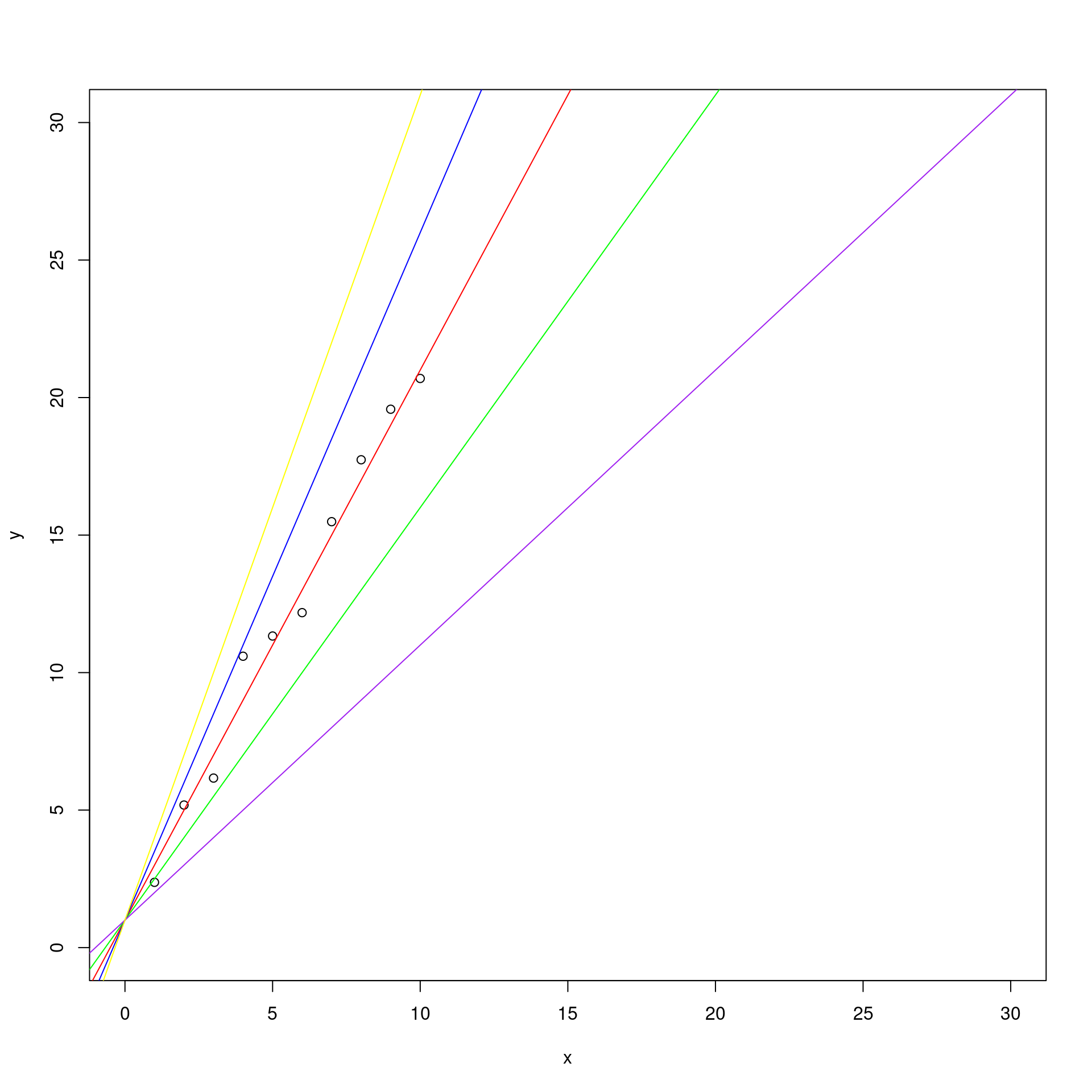

OLS will choose the one with the smallest square of errors \(S(\beta)\).

## creating the data
set.seed( 1 )
# independent variable
x <- 1:10
#   beta0 + i.v. * beta1 + epsilon
y <- 1 + x * 2 + rnorm( n = 10 )

## plotting the data
plot( x , y , ylim = c(0, 30) , xlim = c (0, 30))
abline(a = 1, b = 2 , col = "red")
abline(a = 1, b = 1.5, col = "green")
abline(a = 1, b = 2.5, col = "blue")
abline(a = 1, b = 1, col = "purple")
abline(a = 1, b = 3, col = "yellow")

d1 <- abs( y - (1 + x * 2) )
d2 <- abs( y - (1 + x * 1.5) )
d3 <- abs( y - (1 + x * 2.5) )
d4 <- abs( y - (1 + x * 3) )
d5 <- abs( y - (1 + x) )

segments(x0 = x, y0 = y, x1 = x, y1 = y + d1, col = "red")
segments(x0 = x, y0 = y, x1 = x + d1, y1 = y, col = "red")
segments(x0 = x + d1, y0 = y, x1 = x + d1, y1 = y + d1, col = "red")
segments(x0 = x, y0 = y + d1, x1 = x + d1, y1 = y + d1, col = "red")

segments(x0 = x, y0 = y, x1 = x, y1 = y + d2, col = "green")
segments(x0 = x, y0 = y, x1 = x + d2, y1 = y, col = "green")
segments(x0 = x + d2, y0 = y, x1 = x + d2, y1 = y + d2, col = "green")
segments(x0 = x, y0 = y + d2, x1 = x + d2, y1 = y + d2, col = "green")

segments(x0 = x, y0 = y, x1 = x, y1 = y + d3, col = "blue")
segments(x0 = x, y0 = y, x1 = x + d3, y1 = y, col = "blue")
segments(x0 = x + d3, y0 = y, x1 = x + d3, y1 = y + d3, col = "blue")
segments(x0 = x, y0 = y + d3, x1 = x + d3, y1 = y + d3, col = "blue")

segments(x0 = x, y0 = y, x1 = x, y1 = y + d4, col = "yellow")
segments(x0 = x, y0 = y, x1 = x + d4, y1 = y, col = "yellow")
segments(x0 = x + d4, y0 = y, x1 = x + d4, y1 = y + d4, col = "yellow")
segments(x0 = x, y0 = y + d4, x1 = x + d4, y1 = y + d4, col = "yellow")

segments(x0 = x, y0 = y, x1 = x, y1 = y + d5, col = "purple")
segments(x0 = x, y0 = y, x1 = x + d5, y1 = y, col = "purple")
segments(x0 = x + d5, y0 = y, x1 = x + d5, y1 = y + d5, col = "purple")
segments(x0 = x, y0 = y + d5, x1 = x + d5, y1 = y + d5, col = "purple")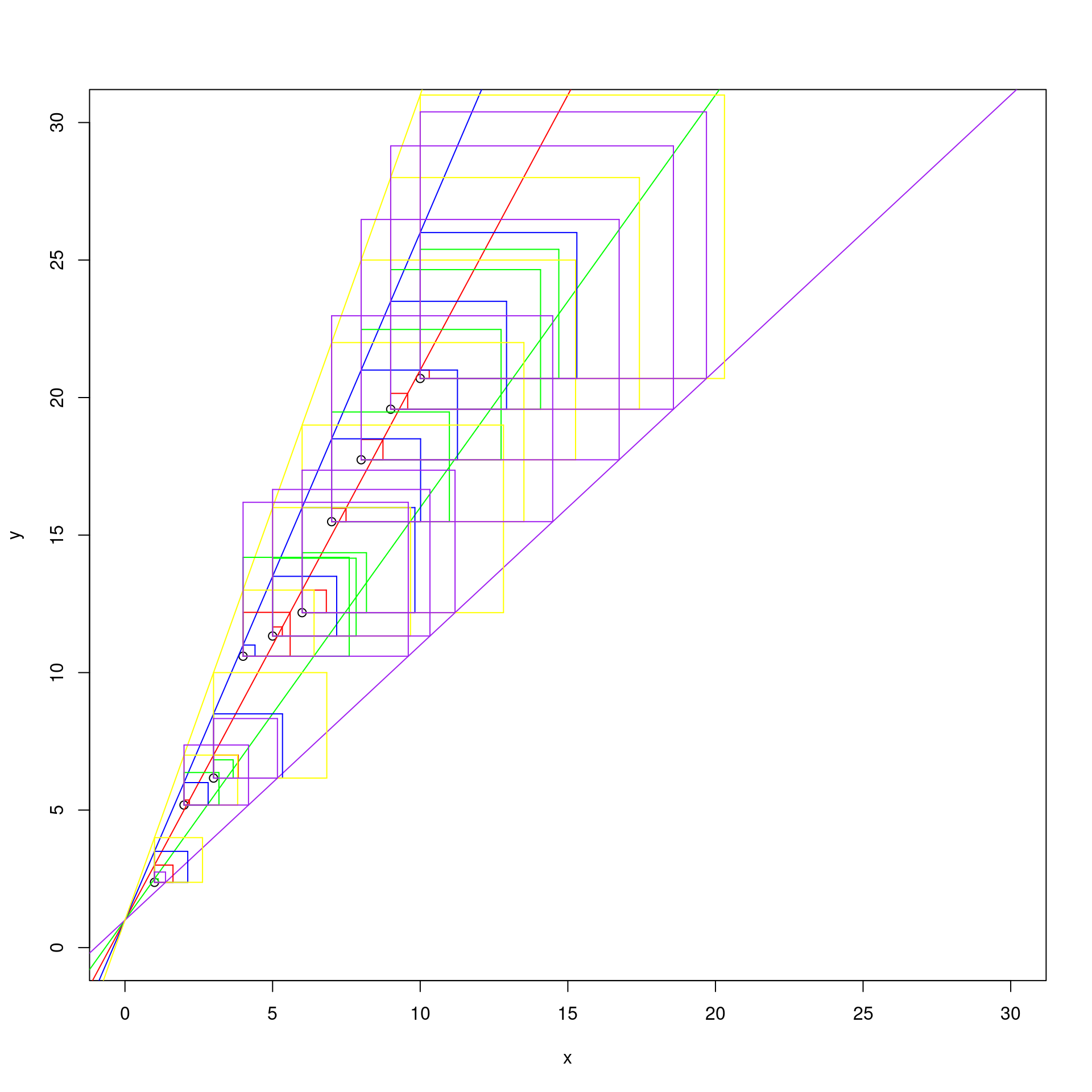

By observing the graph, we can say that is the red one, that has as coefficients \(\beta_0 = 1\) and \(\beta_1 = 2\).

In order to see if analytically is as we observed, we can start with an iterative inefficient function:

find_least_squares <- function( y , x , beta0 , beta1 ) {
  
  # variable for the beta1 that best fits the data
  best_beta <- c(NULL, NULL)
  # variable for memorizing the squared errors
  best_err  <- Inf
  for(int in beta0){
    for( bet in beta1 ){
      yhat <- int + x * bet
      err  <- sum( abs( y - yhat)^2 )
      best_beta[1] <- ifelse( best_err > err,
                           int,
                           best_beta[1])
      best_beta[2] <- ifelse( best_err > err,
                           bet,
                           best_beta[2])
      best_err  <- ifelse( best_err > err,
                           err,
                           best_err)
    }
  }
  
  return( best_beta )
}

print( find_least_squares( y , x, beta0 = seq(from = 0, to = 3, by = 0.1),
                           beta1 = seq(from = 1, to = 3, by = 0.1) ) )

## [1] 0.6 2.1

Let’s try to estimate these values with the standard function of R lm (that does not uses OLS to estimate the coefficients [thanks Marco Tullio Liuzza for the correction]):

mdl <- lm(y ~ x)

print( mdl )

## 
## Call:
## lm(formula = y ~ x)
## 
## Coefficients:
## (Intercept)            x  
##      0.8312       2.0547

As you can see, very similar same results.

plot( x , y )
abline(mdl , col= "red")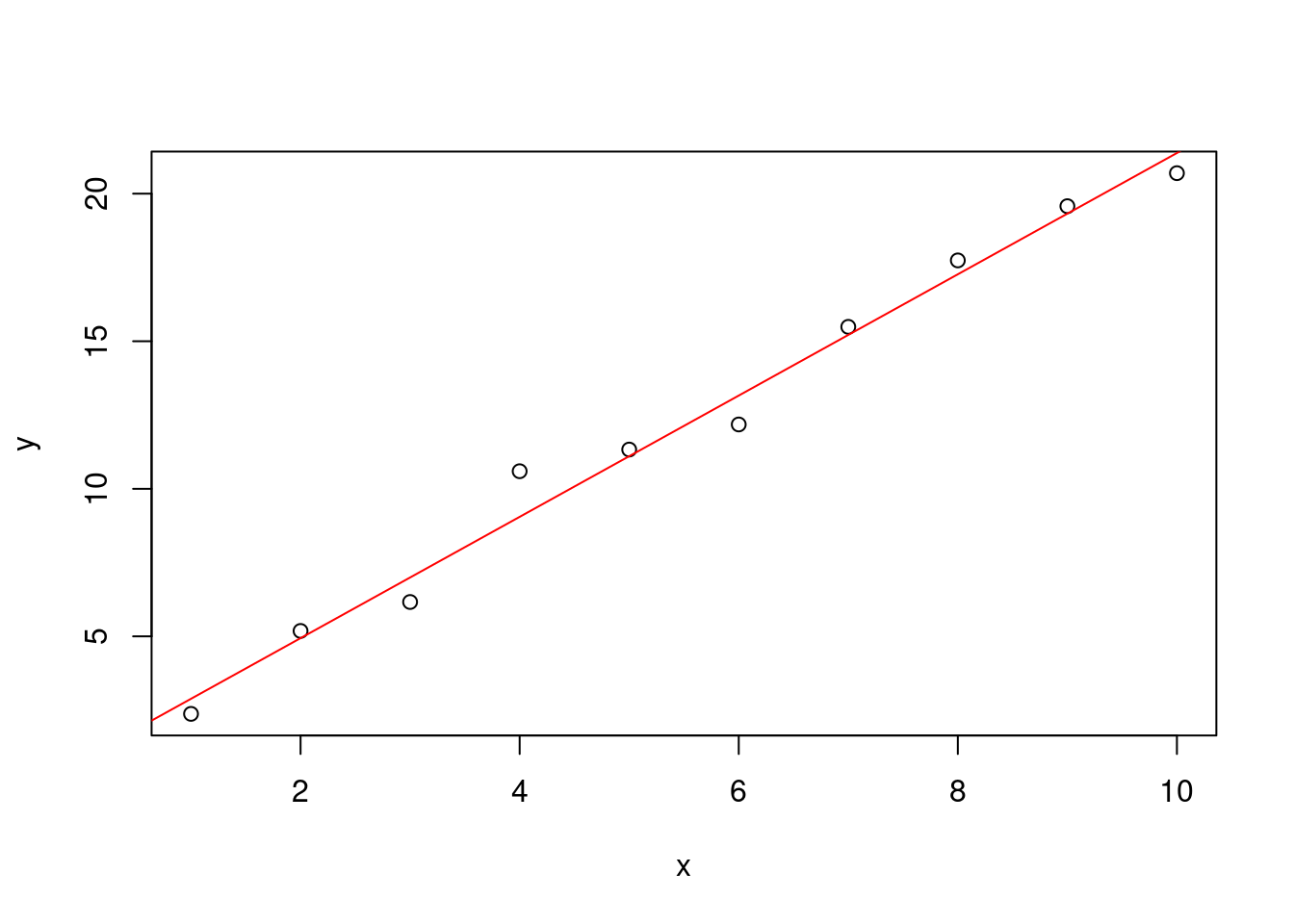

Maximum Likelihood estimation (ML)

In this case we want to maximize the probability of a Likelihood function in describing the data. Therefore, we want to find the values of \(\beta\) that maximize the probability of describing the observed dependent variable \(y\), namely the values of \(\beta\) that, if use din our model, maximize the probability of obtaining the observed data.

Namely, \(\beta = \underset{\beta}{\operatorname{arg max}}~\hat{L}_n(\beta;y)\), where $ L_n(;y)$ is the Likelihood function, that is also an index of goodness of fit of the model (the log-likelihood is often used for model selection).

To better understand how it works, here another interactive, inefficient function (remember that we postulate that our coefficients are distributed along normal distributions):

my_gauss <- function(true_value, sigma, estimate) 1/(sigma*sqrt(2*pi)) *
  exp(- (true_value - estimate)^2/(2*sigma^2))

Thanks to the above function, I will get the likelihood of each parameter, given its true value and the proposed estimate value.

We know that our data were crated with a angular coefficient of 2, therefore this is our true value. We will try different estimate values to see which has the higher likelihood.

find_ML <- function( beta0 , beta1 ) {
  
  # variable for the beta1 that best fits the data
  best_betas <- c(NULL , NULL)
  # variable for memorizing the squared errors
  best_lik  <- -Inf
  
  for(int in beta0){
    for( bet in beta1 ){
      current_lik <- my_gauss(1 , sigma = 1 , int) *
        my_gauss(2 , sigma = 1 , bet)

      best_betas[1] <- ifelse( current_lik > best_lik,
                           int,
                           best_betas[1])
      
      best_betas[2] <- ifelse( current_lik > best_lik,
                           bet,
                           best_betas[2])
      
      best_lik  <- ifelse( current_lik > best_lik,
                           current_lik,
                           best_lik)
    }
  }
  
  return( best_betas )
}

print( find_ML( beta0 = seq(from = 0, to = 3, by = 0.1),
                beta1 = seq(from = 1, to = 3, by = 0.1) ) )

## [1] 1 2

As we can see, also in this case the results are 1 for the intercept and 2 for the angular coefficient.

This methodology can be used in both linear and multilevel linear models.

Restricted (or Residual) Maximum Likelihood (REML)

This method is used in particular in linear models that take into consideration both population- and group-level effects.

As in ML, we want to maximize the Likelihood of the model by finding the best \(\beta\)s parameters. Remember that in linear models all \(\beta\)s are distributed along a normal distribution characterized by a \(\mu\) and \(\sigma\) parameter:

\(\beta \sim N(\mu,\sigma)\)

With this methodology, the computation of the Likelihood of the model is composed by two parts, maximised separately:

1. The Likelihood of \(\mu\) and \(\sigma\) parameters for all group- and population-level effects. \(\leftarrow\) to maximize the likelihood of the \(\mu\) parameter.
2. The Residual Likelihood of only the \(\sigma\) parameters. \(\leftarrow\) to maximize the likelihood of the \(\sigma\) parameter.