library(knitr)
library(captioner)
fig_nums <- captioner()
cod_nums <- captioner( prefix = "Code" )
Some days ago I wrote some notes concerning unbiased estimators, that are the estimators that we commonly use with linear models, and statistical analyses such as ANOVA, linear regression, etc…
Unbiased estimators try to estimate the best unknown but not casual, \(\beta\) coefficients of the independent variables (i.v.) to explain the observed dependent variable \(y\) (d.v.), minimising the error between the variables that can be sampled from the linear model (\(\hat{y}\)) and the observed data (\(y\)).
In other terms, they try to reduce the error between \(y\) and \(\hat{y}\) with different methodologies. We can also say that they look for the values of the coefficients that better “explain the variance”.
Problems with the Unbiased Estimators
That’s great! However, having models that predict so brilliantly the behaviour of a specific sample of data coming from a statistical population, can lead to the problem that the model is not actually so useful in predicting new data and, therefore, it has not really captured the values of the coefficients at a population-level. This is called overfitting.
Overfitting: the production of an analysis that corresponds too closely or exactly to a particular set of data, and may therefore fail to fit additional data or predict future observations reliably
This may also be caused by the use of an excessive number of i.v. in the analysis.
In order to prevent this problem, biased estimators have been proposed.
Biased estimators: algorithms to estimate the values of the coefficients with penalisation coefficients, in order to have coefficients that do not allow the perfect correspondence between \(\hat{y}\) and \(y\).
Concepts that are often used to understand better when a statistical model is a good model are the bias and the variance. Please, note that in this context bias has no relation with cognitive bias, and variance in this context is not the dispersion statistics that we all know.
The bias is the error of the model in fitting the observed data \(y\). A large bias means that the model underfits the sample of data.
x = 1:10
y = x^3/50 + rnorm(10, sd = 1)

plot(x,y)
abline(lm(y~x), col="red")
points(x , x^3/50, type="l", col="green")
legend("top", col = c("red" , "green"), lty = 1,
       legend = c("Underfit" , "Correct fit"))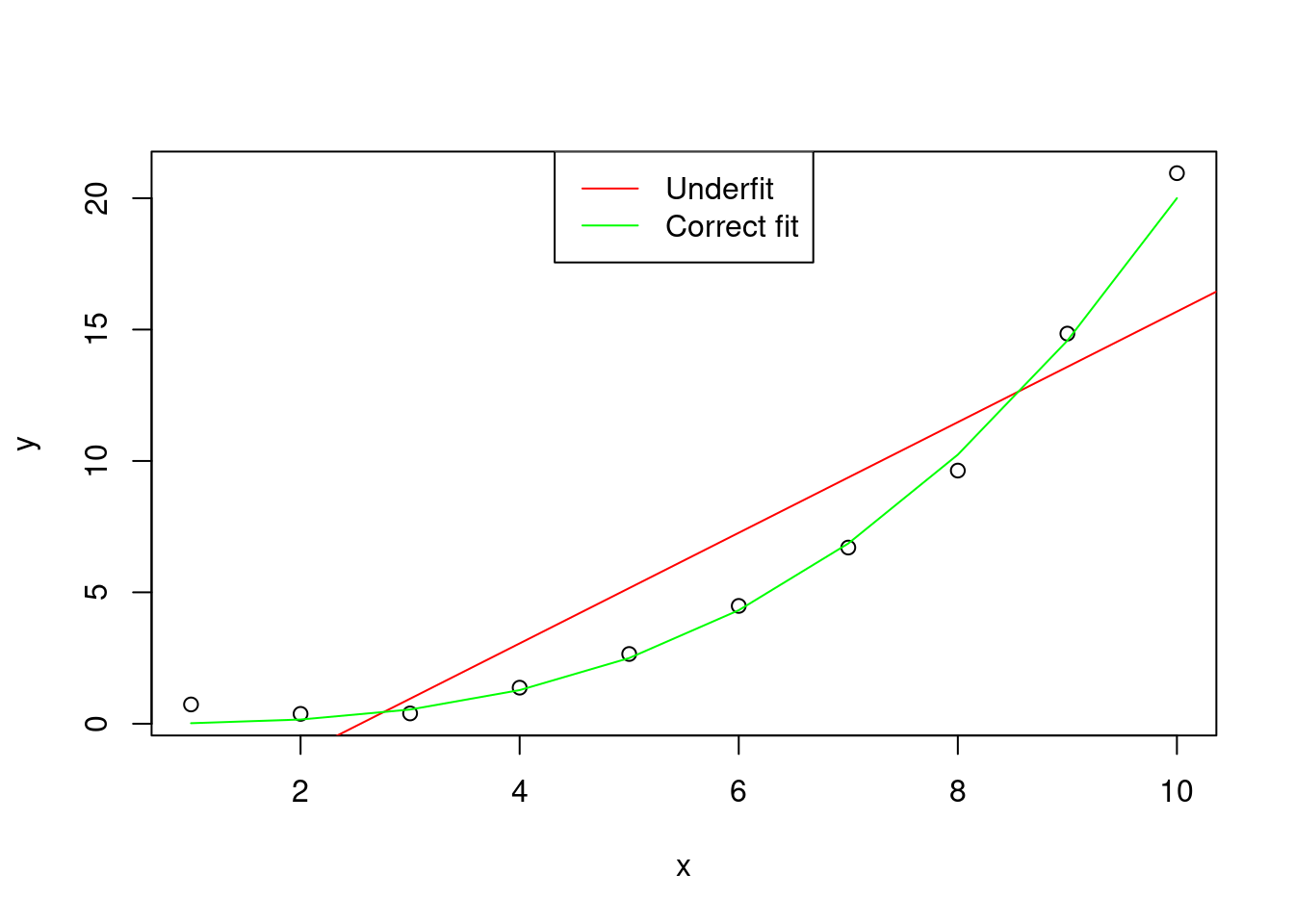
Figure 1: Graphical representation of an hypothetical distribution fitted by two models, one with correct fit (y ~ x^3), and one that underfits the data (y ~ x)
The variance is the error of the model in predicting new data. A large variance means that the model overfits the original sample of data \(y\).
x = seq(from = 1, to = 5, by = 0.1)
y = x^3/100 + cos(x*10)^2

x1 = seq(from = 1, to = 5, by = 0.001)
y1 = x1^3/100 + cos(x1*10)^2

plot(x,y)
points(x1, y1, type="l",  col =" red")
points(x, x^3/100 + mean(cos(x*10)^2), type = "l", col = "green")
legend("topleft", col = c("red" , "green"), lty = 1,
       legend = c("Overfit" , "Correct fit"))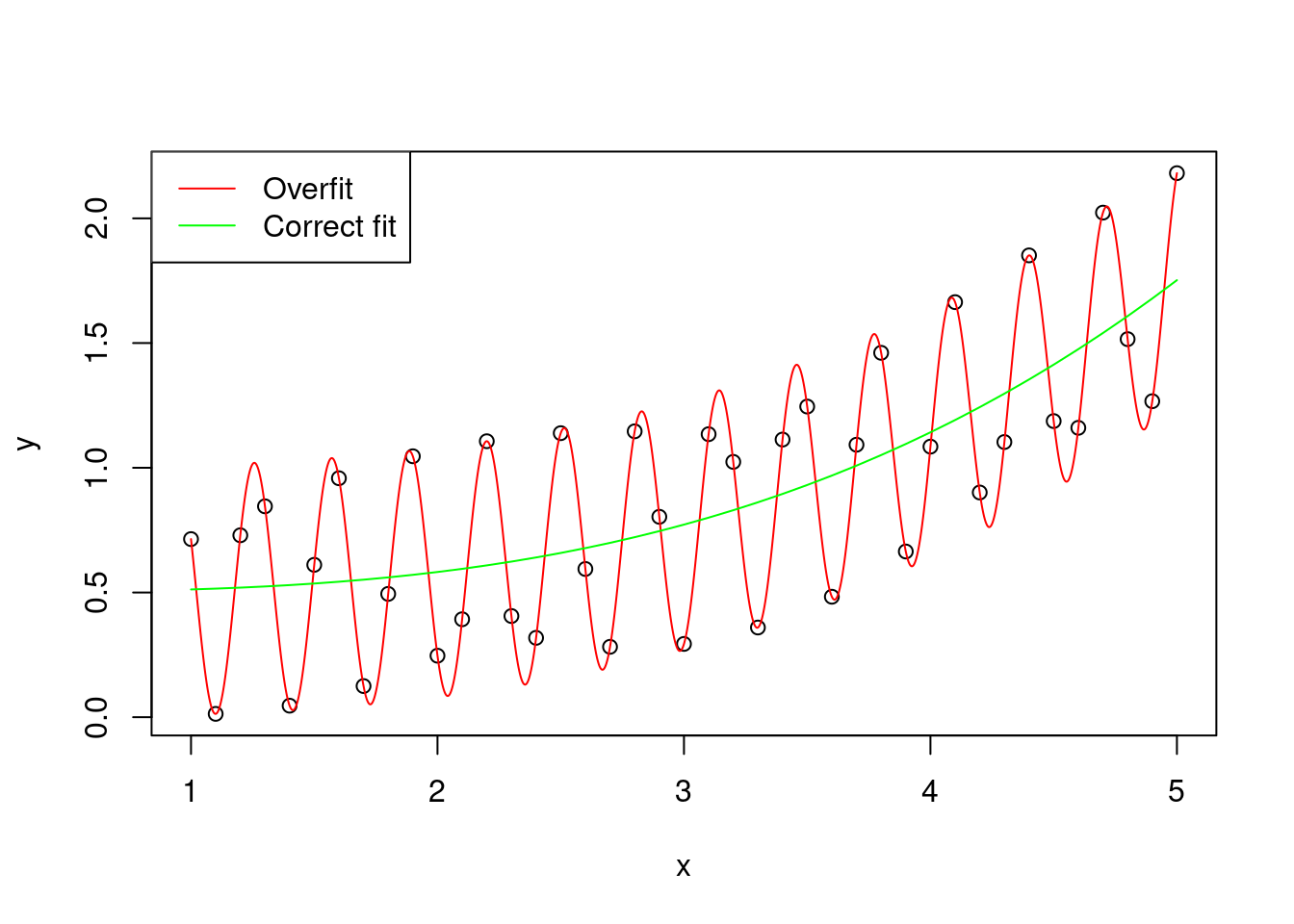
Figure 2: Graphical representation of an hypothetical distribution fitted by two models, one with correct fit (y ~ x^3), and one that overfits the data (y ~ x^3 + cos(x * 10)^2)
(to be honest, the overfitted curve is obtained by using exactly y ~ x^3 + cos(x * 10)^2, but for simplicity let’s pretend that the cosine part is just random variation)
A good model should have low bias and low variance, finding the trade-off between them.
x = 1:100
y = x^5 / 1e10

plot( x = 1:100 , y , type = "l" , col = "red")
points( x = 100:1 , y = y , type = "l", col = "blue")
points( x = 1:100 , y = y + y[100:1] + 0.1 , type = "l" , col = "green")
legend("top", col = c("red" , "blue" , "green"), lty = 1, legend = c("Bias" , "Variance" , "Error trade-Off"))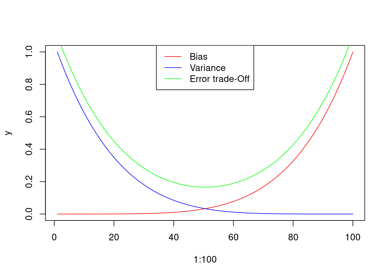
Figure 3: Graphical representation of the Bias and Variance errors of the model, and hypothetical trade-off curve. Please note that the Trade-off curve has been displaced for a better visualization
The most famous among the biased estimators are the:
- Ridge regression (a.k.a. L2 regularization)
- Lasso regression (a.k.a. L1 regularization)
Ridge regression
Ridge regression tries to find the best coefficients (\(\beta\)s) that describe our observed sample of data (\(y\)), penalising the computation of the coefficients with a coefficient \(\lambda\).
Therefore, the idea is to find the \(\beta\)s of the model that best fit the data, with an additional penalysing term \(\lambda\).
\(\beta = \underset{\beta}{\operatorname{arg min}}~S(\beta, \lambda)\)
where
\(S(\beta, \lambda) = \sum_{i=1}^{n} \frac{1}{2} ( y_i - \sum_{j=1}^p x_{i,j} \beta_{j})^2+\lambda \sum_{j=1}^p \beta_j^2\)
\(\lambda\) is the complexity parameter, and penalises the \(\beta\)s, limiting overfitting and shrinking large \(\beta\)s.
In order to better understand how ridge regression works, we can use an iterative, inefficient, and so simplified to be simply wrong, function just to have an idea concerning how ridge regression works.
In this function we create some random data gaussianally distributed, coming from a linear model with mean 1 (\(\beta_0\)) and regressor \(\beta_1 = 2\).
The same data used for unbiased estimators.
We set our \(\lambda\) to 0.1.
## creating the data
set.seed( 1 )
# independent variable
x <- 1:10
#   beta0 + i.v. * beta1 + epsilon
y <- 1 + x * 2 + rnorm( n = 10 )

find_ridge_least_squares <- function( y , x , beta0 , beta1 , lambda ) {

  # variable for the beta1 that best fits the data
  best_beta <- c(NULL, NULL)
  # variable for memorizing the squared errors
  best_err  <- Inf
  for(int in beta0){
    for( bet in beta1 ){
      yhat <- int + x * bet
      err  <- ( sum( ( y - yhat)^2 ) / 2 ) + ( lambda * ( int^2 + bet^2 ) )
      best_beta[1] <- ifelse( best_err > err,
                           int,
                           best_beta[1])
      best_beta[2] <- ifelse( best_err > err,
                           bet,
                           best_beta[2])
      best_err  <- ifelse( best_err > err,
                           err,
                           best_err)
    }
  }

  return( best_beta )
}

print(
  find_ridge_least_squares( y ,
                            x,
                            beta0 = seq(from = 0, to = 3, by = 0.01),
                            beta1 = seq(from = 1, to = 3, by = 0.01),
                            lambda = 0.01 )
)
## [1] 0.80 2.06Code 1: Exemplification code for a ridge regression
The estimations are not so far from the real values. However, let’s
see how the real function works, in library glmnet:
library("glmnet")## Carico il pacchetto richiesto: Matrix## Loaded glmnet 4.0-2fit <- glmnet(y = y, x = cbind(1,x),
lambda = 0.01, alpha = 0)
print( coef( fit ) )## 3 x 1 sparse Matrix of class "dgCMatrix"
## s0
## (Intercept) 0.8501507
## .
## x 2.0512822Code 2: Use of glmnet for ridge regression
The minimisation problem has a unique solution:
\(\beta = (X^TX + \lambda I)^{-1}X^Ty\)
X = cbind( 1 , x )

solve( t(X) %*% X + 0.01 * diag(2) ) %*% t(X) %*% y
## [,1]
## 0.8286793
## x 2.0550354Code 3: Matrix computation for Ridge regression
In this case we can see that the algorithms used in the glmnet function
and in the matrix computation are different.
glmnet is a complex function that allows to compute Ridge regression (alpha = 0),
Lasso regression (alpha = 1) and Elasticnet regression (alpha \(\in\) [0, 1]),
and probably it is using
algorithms that are more advanced than the classical ones that I am using here.
Lasso regression
The Least Absolute Shrinkage and Selection Operator (Lasso) regression is very similar to the Ridge regression.
In fact, it uses the \(\lambda\) coefficient of penalisation already seen in the Ridge regression.
Therefore, the minimisation problem is always:
\(\beta = \underset{\beta}{\operatorname{arg min}}~S(\beta, \lambda)\)
but the \(S\) function changes:
\(S(\beta, \lambda) = \frac{1}{n}\sum_{i=1}^{n} ( y_i - \sum_{j=1}^p x_{i,j} \beta_{j})^2+\frac{\lambda}{2} \sum_{j=1}^p |\beta_j|\)
find_lasso_least_squares <- function( y , x , beta0 , beta1 , lambda ) {

  # variable for the beta1 that best fits the data
  best_beta <- c(NULL, NULL)
  # variable for memorizing the squared errors
  best_err  <- Inf
  for(int in beta0){
    for( bet in beta1 ){
      yhat <- int + x * bet
      err  <- ( sum( ( y - yhat)^2 ) / ( length(yhat) ) ) +
        ( lambda / 2 * abs( int + bet ) )
      best_beta[1] <- ifelse( best_err > err,
                           int,
                           best_beta[1])
      best_beta[2] <- ifelse( best_err > err,
                           bet,
                           best_beta[2])
      best_err  <- ifelse( best_err > err,
                           err,
                           best_err)
    }
  }

  return( best_beta )
}

print(
  find_lasso_least_squares( y ,
                            x,
                            beta0 = seq(from = 0, to = 3, by = 0.01),
                            beta1 = seq(from = 1, to = 3, by = 0.01),
                            lambda = 0.01 )
)
## [1] 0.80 2.06Code 4: Exemplification code for a Lasso regression
fit <- glmnet(y = y, x = cbind(1,x),
              lambda = 0.01)

print( coef( fit ) )
## 3 x 1 sparse Matrix of class "dgCMatrix"
## s0
## (Intercept) 0.850325
## .
## x 2.051251Code 5: Use of glmnet for Lasso regression
The minimisation problem can be divided in two steps:
- finding the \(\beta\)s with OLS (\(\beta = (X^TX)^{-1}X^Ty\))
- applying the Lasso penalisation (\((1+N \frac{\lambda}{2})^{-1}\))
\(\beta = (1+N \frac{\lambda}{2})^{-1}[(X^TX)^{-1}X^Ty]\)
X = cbind( 1 , x )

(1 + nrow(X) * 0.01 / 2)^(-1) *
solve( t(X) %*% X ) %*% t(X) %*% y
## [,1]
## 0.7915966
## x 1.9568877Also in this case the results are different from the glmnet function.
I suspect that in the glmnet function they are using more advanced versions
of the Lasso regression.