This post is based on Rasmus Bååth’s robust correlation model in JAGS, and Adrian Baez-Ortega conversion in Stan.
For their original contributions, see:
- Bayesian correlation in JAGS
- Robust Bayesian Correlation in JAGS
- Robust Bayesian Correlation in Stan
In this post, I start from the Rasmus Bååth and Adrian Baez-Ortega work, to extend it later, by adding the possibility to obtain Savage-Dickey density ratio Bayes Factors and the possibility to compute multiple correlation with a single function (instead to compute many one-to-one correlations, saving time and computational resources).
The Basic Idea
In order to compute the correlation between two normally-distributed variables
\(y \sim \mathcal{N}(\mu_y,\sigma^2_y)\) \(x \sim \mathcal{N}(\mu_x,\sigma^2_x)\)
set.seed(4)

x <- rnorm(100, mean = 10, sd = 5)
y <- x * 0.7 + rnorm(100, mean = 3.7, sd = pi/2)

dat <- data.frame(x , y)

g1 <- ggplot( dat, aes(y = y, x = x) )+
  geom_density_2d()+
  geom_point()+
  xlim(c(-5, 30))+
  ylim(c(-5, 30))

ggMarginal(g1, type = "histogram", bins = 20)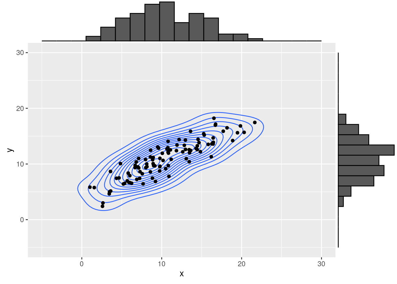
The brilliant idea behind this is that two variables that correlate they obviously share some covariance, that is composed by the variances and their correlation.
From the covariance matrix to the correlation matrix
Therefore, these two independent-but-correlating normal distributions, can be seen as a multinormal distribution with their own variance-covariance matrix (a.k.a covariance matrix).
Thus, our dataset becomes:
\([y, x] \sim \mathcal{MN}(M, \Omega)\)
where \(M = [\mu_y, \mu_x]\) is the vector of the means, and
\[\Omega = \left[\begin{array}{cc} \sigma_y^2 & \sigma_x \sigma_y \rho_{x,y}\\ \sigma_x \sigma_y \rho_{x,y} & \sigma_x^2 \end{array}\right] \]
(in order to simplify the notation, \(\sigma\) will be the variance and not, as usual, the standard deviation).
The variance-covariance matrix \(\Omega\) can be computed starting from the diagonal matrix of variances \(\Sigma\) and the correlation matrix \(R\)
\[\Omega = \Sigma \times R \times \Sigma = \left[\begin{array}{cc} \sigma_y & 0\\ 0 & \sigma_x \end{array}\right] \times \left[\begin{array}{cc} 1 & \rho_{x,y}\\ \rho_{x,y} & 1 \end{array}\right] \times \left[\begin{array}{cc} \sigma_y & 0\\ 0 & \sigma_x \end{array}\right] \]
Just to confirm that everything its written here is correct, some math:
# std dev for    x  y    with square-elevation to have the variances
Sigma <- diag( c(5, pi/2)^2 )

kable(Sigma, caption = "Variances diagonal matrix")
## Warning in kable_pipe(x = structure(c("25", "0", "0.000000", "2.467401"), .Dim =
## c(2L, : The table should have a header (column names)| 25 | 0.000000 |
| 0 | 2.467401 |
R <- matrix( c(1  , 0.7,
               0.7, 1  ),
             byrow = TRUE,
             ncol = 2 )

kable(R, caption = "Correlation matrix")
## Warning in kable_pipe(x = structure(c("1.0", "0.7", "0.7", "1.0"), .Dim =
## c(2L, : The table should have a header (column names)| 1.0 | 0.7 |
| 0.7 | 1.0 |
kable(Sigma %*% R %*% Sigma, digits = 2, caption = "Covariance matrix")## Warning in kable_pipe(x = structure(c("625.00", "43.18", "43.18", "6.09": The
## table should have a header (column names)| 625.00 | 43.18 |
| 43.18 | 6.09 |
kable(cov2cor(Sigma %*% R %*% Sigma),
      caption = "If everything is correct, we should have our correlation matrix back")
## Warning in kable_pipe(x = structure(c("1.0", "0.7", "0.7", "1.0"), .Dim =
## c(2L, : The table should have a header (column names)| 1.0 | 0.7 |
| 0.7 | 1.0 |
Well, yes, nothing spectacular, but at least we are sure that the math is OK.
The prior distributions from the Rasmus Bååth work and a normal Bayesian correlation
In order to obtain a posterior distribution for \(\rho_{x,y}\), in our Bayesian code we should estimate the posterior distribution for:
\(M\), that for Rasmus Bååth suggestions, each element can be non-informative \(\mu \sim \mathcal{N}(0, 1000)\)
The \(\Sigma\) diagonal matrix, that with an non-informative prior each element would be: \(\sigma \sim \mathcal{U}(0, 1000)\)
\(rho\), whose non-informative distribution would be \(\rho \sim \mathcal{U}(-1, 1)\)
Therefore, the Stan code is:
stancode1 <-"
data {
    int<lower=1> N;  // number of observations
    vector[2] x[N];  // input data: rows are observations, columns are the two variables
}

parameters {
    vector[2] mu;                 // means vector
    real<lower=0> sigma[2];       // variances vector
    real<lower=-1, upper=1> rho;    // correlation coefficient
}

transformed parameters {
    // Covariance matrix
    cov_matrix[2] cov = [[      sigma[1] ^ 2       , sigma[1] * sigma[2] * rho],
                         [sigma[1] * sigma[2] * rho,       sigma[2] ^ 2       ]];
}

model {
    // Likelihood
    // Bivariate Student's t-distribution instead of normal for robustness
    x ~ multi_normal(mu, cov);

    // Noninformative priors on all parameters
    sigma ~ uniform(0, 1000);
    mu ~ normal(0, 1000);
    rho ~ uniform(-1,1);//non informative prior between -1 and 1
}

generated quantities {
    // Random samples from the estimated bivariate normal distribution (for assessment of fit)
    vector[2] x_rand;
    x_rand = multi_normal_rng(mu, cov);
}"
… and to call it, you just need to prepare you data list and run the analysis
library(rstan)## Carico il pacchetto richiesto: StanHeaders## rstan (Version 2.21.2, GitRev: 2e1f913d3ca3)## For execution on a local, multicore CPU with excess RAM we recommend calling
## options(mc.cores = parallel::detectCores()).
## To avoid recompilation of unchanged Stan programs, we recommend calling
## rstan_options(auto_write = TRUE)library(bayesplot)## This is bayesplot version 1.7.2## - Online documentation and vignettes at mc-stan.org/bayesplot## - bayesplot theme set to bayesplot::theme_default()## * Does _not_ affect other ggplot2 plots## * See ?bayesplot_theme_set for details on theme settingdata.list <- list(
x = cbind( x, y ),
N = nrow( dat )
)
mdlCor1 <- stan(
model_code = stancode1,
data = data.list,
pars = "rho",
refresh = 0
)## Trying to compile a simple C file## Running /usr/lib/R/bin/R CMD SHLIB foo.c
## gcc -std=gnu99 -I"/usr/share/R/include" -DNDEBUG -I"/home/michele/R/x86_64-pc-linux-gnu-library/4.0/Rcpp/include/" -I"/home/michele/R/x86_64-pc-linux-gnu-library/4.0/RcppEigen/include/" -I"/home/michele/R/x86_64-pc-linux-gnu-library/4.0/RcppEigen/include/unsupported" -I"/home/michele/R/x86_64-pc-linux-gnu-library/4.0/BH/include" -I"/home/michele/R/x86_64-pc-linux-gnu-library/4.0/StanHeaders/include/src/" -I"/home/michele/R/x86_64-pc-linux-gnu-library/4.0/StanHeaders/include/" -I"/home/michele/R/x86_64-pc-linux-gnu-library/4.0/RcppParallel/include/" -I"/home/michele/R/x86_64-pc-linux-gnu-library/4.0/rstan/include" -DEIGEN_NO_DEBUG -DBOOST_DISABLE_ASSERTS -DBOOST_PENDING_INTEGER_LOG2_HPP -DSTAN_THREADS -DBOOST_NO_AUTO_PTR -include '/home/michele/R/x86_64-pc-linux-gnu-library/4.0/StanHeaders/include/stan/math/prim/mat/fun/Eigen.hpp' -D_REENTRANT -DRCPP_PARALLEL_USE_TBB=1 -fpic -g -O2 -fdebug-prefix-map=/build/r-base-8T8CYO/r-base-4.0.3=. -fstack-protector-strong -Wformat -Werror=format-security -Wdate-time -D_FORTIFY_SOURCE=2 -g -c foo.c -o foo.o
## In file included from /home/michele/R/x86_64-pc-linux-gnu-library/4.0/RcppEigen/include/Eigen/Core:88,
## from /home/michele/R/x86_64-pc-linux-gnu-library/4.0/RcppEigen/include/Eigen/Dense:1,
## from /home/michele/R/x86_64-pc-linux-gnu-library/4.0/StanHeaders/include/stan/math/prim/mat/fun/Eigen.hpp:13,
## from <command-line>:
## /home/michele/R/x86_64-pc-linux-gnu-library/4.0/RcppEigen/include/Eigen/src/Core/util/Macros.h:613:1: error: unknown type name ‘namespace’
## 613 | namespace Eigen {
## | ^~~~~~~~~
## /home/michele/R/x86_64-pc-linux-gnu-library/4.0/RcppEigen/include/Eigen/src/Core/util/Macros.h:613:17: error: expected ‘=’, ‘,’, ‘;’, ‘asm’ or ‘__attribute__’ before ‘{’ token
## 613 | namespace Eigen {
## | ^
## In file included from /home/michele/R/x86_64-pc-linux-gnu-library/4.0/RcppEigen/include/Eigen/Dense:1,
## from /home/michele/R/x86_64-pc-linux-gnu-library/4.0/StanHeaders/include/stan/math/prim/mat/fun/Eigen.hpp:13,
## from <command-line>:
## /home/michele/R/x86_64-pc-linux-gnu-library/4.0/RcppEigen/include/Eigen/Core:96:10: fatal error: complex: File o directory non esistente
## 96 | #include <complex>
## | ^~~~~~~~~
## compilation terminated.
## make: *** [/usr/lib/R/etc/Makeconf:172: foo.o] Errore 1kable( summary(mdlCor1)[[1]] , digits = 3,
caption = "Posterior distribution for the rho parameter")| mean | se_mean | sd | 2.5% | 25% | 50% | 75% | 97.5% | n_eff | Rhat | |
|---|---|---|---|---|---|---|---|---|---|---|
| rho | 0.879 | 0.001 | 0.023 | 0.827 | 0.866 | 0.881 | 0.896 | 0.919 | 1868.711 | 1.000 |
| lp__ | -298.518 | 0.039 | 1.569 | -302.417 | -299.336 | -298.207 | -297.344 | -296.436 | 1581.159 | 1.002 |
mcmc_combo(
  mdlCor1,
  pars = "rho"
)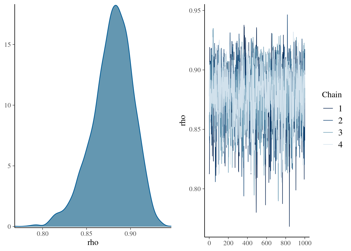
Figure 1: Density and trace plot for our rho parameter of the first bayesian correlation in stan
Ok, so here we have some results.
I am not showing you how to check if the model is ok, etc… etc… Rasmus Bååth did a great job, so you might want to take a look at his page.
The Bayesian Robust Correlation
Anyway, the best part of the Rasmus Bååth work was to enhance the correlation concept towards a robust correlation that, at the best of my knowledge, has no similarities with any “traditional” correlation coefs.
Robust: more resistent to outliers
Therefore, as it is usually done to have robust linear models in Bayesian Statistics, the prior for our observed variables is not anymore a Normal distribution, but a Student’s t distribution with unknown \(\nu\) degrees of freedom.
The Student’s t distribution has strong connections with the Normal distribution but, changing its degrees of freedom (\(\nu\)), the tails can allow more probability at the extremes (smaller degrees of freedom), or less probability (larger degrees of freedom). It is known that a Student’s t distribution with \(\nu \to + \inf\) is a Normal distribution.
Smaller \(\nu\) it is allowed that extreme values are further from the center of the distribution (namely, the \(\mu\) of the Student’s t distribution is more resilient to outliers), while greater \(\nu\) values makes \(\mu\) more dependent to extreme values.
Consequently, in the code we changed these prior distributions:
- \(M\), \(\mu \sim \mathcal{Student~t}(\nu, 0, 1000)\)
- \(\nu \sim \mathcal{U}(0, 1000)\)
stancode2 <-"
data {
    int<lower=1> N;  // number of observations
    vector[2] x[N];  // input data: rows are observations, columns are the two variables
}

parameters {
    vector[2] mu;                 // mean vector of the marginal t distributions
    real<lower=0> sigma[2];       // variance vector of the marginal t distributions
    real<lower=1> nu;             // degrees of freedom of the marginal t distributions
    real<lower=-1, upper=1> rho;  // correlation coefficient
}

transformed parameters {
    // Covariance matrix
    cov_matrix[2] cov = [[      sigma[1] ^ 2       , sigma[1] * sigma[2] * rho],
                         [sigma[1] * sigma[2] * rho,       sigma[2] ^ 2       ]];
}

model {
    // Likelihood
    // Bivariate Student's t-distribution instead of normal for robustness
    x ~ multi_student_t(nu, mu, cov);

    // Noninformative priors on all parameters
    sigma ~ uniform(0, 1000);
    mu ~ normal(0, 1000);
    nu ~ uniform(0,1000);
    rho ~ uniform(-1,1);//non informative prior between -1 and 1
}

generated quantities {
    // Random samples from the estimated bivariate t-distribution (for assessment of fit)
    vector[2] x_rand;
    x_rand = multi_student_t_rng(nu, mu, cov);
}
"
and these are the new results:
mdlCor2 <- stan(
  model_code = stancode2,
  data = data.list,
  pars = c("rho","nu"),
  refresh = 0
)
## Trying to compile a simple C file## Running /usr/lib/R/bin/R CMD SHLIB foo.c
## gcc -std=gnu99 -I"/usr/share/R/include" -DNDEBUG -I"/home/michele/R/x86_64-pc-linux-gnu-library/4.0/Rcpp/include/" -I"/home/michele/R/x86_64-pc-linux-gnu-library/4.0/RcppEigen/include/" -I"/home/michele/R/x86_64-pc-linux-gnu-library/4.0/RcppEigen/include/unsupported" -I"/home/michele/R/x86_64-pc-linux-gnu-library/4.0/BH/include" -I"/home/michele/R/x86_64-pc-linux-gnu-library/4.0/StanHeaders/include/src/" -I"/home/michele/R/x86_64-pc-linux-gnu-library/4.0/StanHeaders/include/" -I"/home/michele/R/x86_64-pc-linux-gnu-library/4.0/RcppParallel/include/" -I"/home/michele/R/x86_64-pc-linux-gnu-library/4.0/rstan/include" -DEIGEN_NO_DEBUG -DBOOST_DISABLE_ASSERTS -DBOOST_PENDING_INTEGER_LOG2_HPP -DSTAN_THREADS -DBOOST_NO_AUTO_PTR -include '/home/michele/R/x86_64-pc-linux-gnu-library/4.0/StanHeaders/include/stan/math/prim/mat/fun/Eigen.hpp' -D_REENTRANT -DRCPP_PARALLEL_USE_TBB=1 -fpic -g -O2 -fdebug-prefix-map=/build/r-base-8T8CYO/r-base-4.0.3=. -fstack-protector-strong -Wformat -Werror=format-security -Wdate-time -D_FORTIFY_SOURCE=2 -g -c foo.c -o foo.o
## In file included from /home/michele/R/x86_64-pc-linux-gnu-library/4.0/RcppEigen/include/Eigen/Core:88,
## from /home/michele/R/x86_64-pc-linux-gnu-library/4.0/RcppEigen/include/Eigen/Dense:1,
## from /home/michele/R/x86_64-pc-linux-gnu-library/4.0/StanHeaders/include/stan/math/prim/mat/fun/Eigen.hpp:13,
## from <command-line>:
## /home/michele/R/x86_64-pc-linux-gnu-library/4.0/RcppEigen/include/Eigen/src/Core/util/Macros.h:613:1: error: unknown type name ‘namespace’
## 613 | namespace Eigen {
## | ^~~~~~~~~
## /home/michele/R/x86_64-pc-linux-gnu-library/4.0/RcppEigen/include/Eigen/src/Core/util/Macros.h:613:17: error: expected ‘=’, ‘,’, ‘;’, ‘asm’ or ‘__attribute__’ before ‘{’ token
## 613 | namespace Eigen {
## | ^
## In file included from /home/michele/R/x86_64-pc-linux-gnu-library/4.0/RcppEigen/include/Eigen/Dense:1,
## from /home/michele/R/x86_64-pc-linux-gnu-library/4.0/StanHeaders/include/stan/math/prim/mat/fun/Eigen.hpp:13,
## from <command-line>:
## /home/michele/R/x86_64-pc-linux-gnu-library/4.0/RcppEigen/include/Eigen/Core:96:10: fatal error: complex: File o directory non esistente
## 96 | #include <complex>
## | ^~~~~~~~~
## compilation terminated.
## make: *** [/usr/lib/R/etc/Makeconf:172: foo.o] Errore 1## Warning: There were 3290 divergent transitions after warmup. See
## http://mc-stan.org/misc/warnings.html#divergent-transitions-after-warmup
## to find out why this is a problem and how to eliminate them.## Warning: Examine the pairs() plot to diagnose sampling problems## Warning: Bulk Effective Samples Size (ESS) is too low, indicating posterior means and medians may be unreliable.
## Running the chains for more iterations may help. See
## http://mc-stan.org/misc/warnings.html#bulk-esskable( summary(mdlCor2)[[1]] , digits = 3,
caption = "Posterior distribution for the rho and nu parameters")| mean | se_mean | sd | 2.5% | 25% | 50% | 75% | 97.5% | n_eff | Rhat | |
|---|---|---|---|---|---|---|---|---|---|---|
| rho | 0.878 | 0.001 | 0.023 | 0.825 | 0.865 | 0.879 | 0.894 | 0.916 | 328.758 | 1.020 |
| nu | 514.408 | 13.514 | 273.050 | 54.721 | 284.376 | 512.978 | 752.251 | 973.033 | 408.216 | 1.019 |
| lp__ | -362.048 | 0.070 | 1.856 | -366.584 | -363.054 | -361.739 | -360.725 | -359.387 | 709.467 | 1.012 |
mcmc_combo(
  mdlCor2,
  pars = c("rho", "nu")
)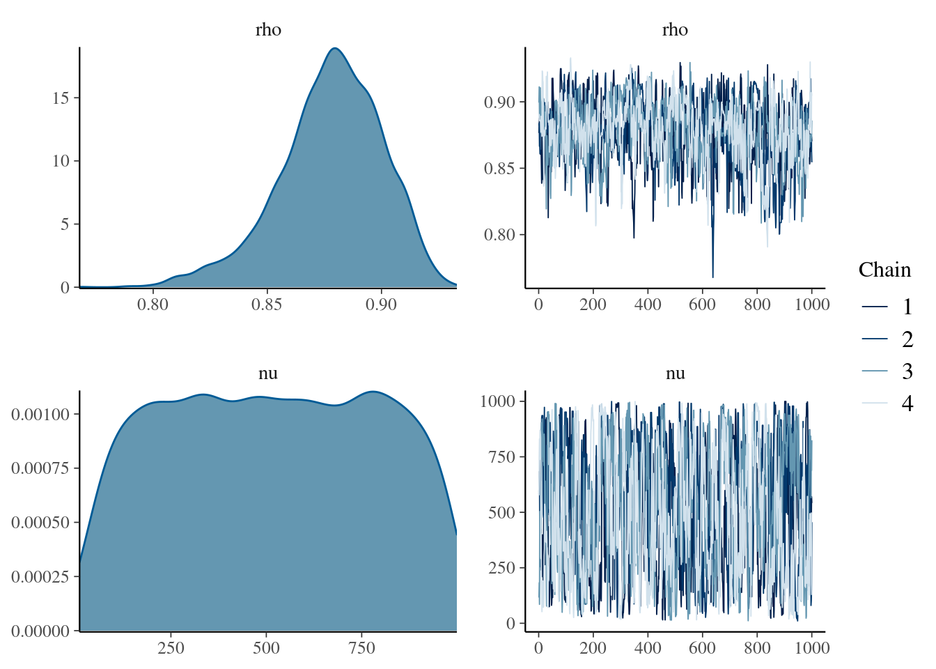
Well, the two distributions are directly coming from random normal distributions, so there should not be big differences between this robust and the non-robust version.
However, here we gain the \(\nu\) (nu) parameter, that as Krushcke said (in one of its books), it might be an index of normality of our distributions.
We all know that a Student’s t distribution with \(\Inf\) degrees of freedom is basically the same as a Normal distribution. Therefore, if our \(\nu\) distribution stretched toward small numbers it should be an index that our distributions are not parametrically distributed (in fact, a Cauchy distribution is a Student’s t distribution with 1 degree of freedom).
The Bayesian Robust Correlation: degrees of freedom dependent from the number of observations
However, why should \(\nu\) be unknown?
We all know that, for an extension of the central limit theorem, the biggest the sample, the more “certain” is the mean.
Central Limit Theorem: when independent random variables are added, their properly normalized sum tends toward a normal distribution
Therefore, it might be reasonable to establish some relation between the number of observations and \(\nu\).
Here it starts my personal contribution, that you can also find in my github.
I have decided that the number of degrees of freedom are equal to the number of observations divided by 10 plus 1.
stancode3 <-"
data {
    int<lower=1> N;  // number of observations
    vector[2] x[N];  // input data: rows are observations, columns are the two variables
}

parameters {
    vector[2] mu;                 // mean vector of the marginal t distributions
    real<lower=0> sigma[2];       // variance vector of the marginal t distributions
    real<lower=-1, upper=1> rho;  // correlation coefficient
}

transformed parameters {
    // degrees of freedom of the marginal t distributions
    real<lower=1> nu = (N / 10.0) + 1;

    // Covariance matrix
    cov_matrix[2] cov = [[      sigma[1] ^ 2       , sigma[1] * sigma[2] * rho],
                         [sigma[1] * sigma[2] * rho,       sigma[2] ^ 2       ]];
}

model {
    // Likelihood
    // Bivariate Student's t-distribution instead of normal for robustness
    x ~ multi_student_t(nu, mu, cov);

    // Noninformative priors on all parameters
    sigma ~ uniform(0, 1000);
    mu ~ normal(0, 1000);
    rho ~ uniform(-1,1);//non informative prior between -1 and 1
}

generated quantities {
    // Random samples from the estimated bivariate t-distribution (for assessment of fit)
    vector[2] x_rand;
    x_rand = multi_student_t_rng(nu, mu, cov);
}
"

mdlCor3 <- stan(
  model_code = stancode3,
  data = data.list,
  pars = "rho",
  refresh = 0
)
## Trying to compile a simple C file## Running /usr/lib/R/bin/R CMD SHLIB foo.c
## gcc -std=gnu99 -I"/usr/share/R/include" -DNDEBUG -I"/home/michele/R/x86_64-pc-linux-gnu-library/4.0/Rcpp/include/" -I"/home/michele/R/x86_64-pc-linux-gnu-library/4.0/RcppEigen/include/" -I"/home/michele/R/x86_64-pc-linux-gnu-library/4.0/RcppEigen/include/unsupported" -I"/home/michele/R/x86_64-pc-linux-gnu-library/4.0/BH/include" -I"/home/michele/R/x86_64-pc-linux-gnu-library/4.0/StanHeaders/include/src/" -I"/home/michele/R/x86_64-pc-linux-gnu-library/4.0/StanHeaders/include/" -I"/home/michele/R/x86_64-pc-linux-gnu-library/4.0/RcppParallel/include/" -I"/home/michele/R/x86_64-pc-linux-gnu-library/4.0/rstan/include" -DEIGEN_NO_DEBUG -DBOOST_DISABLE_ASSERTS -DBOOST_PENDING_INTEGER_LOG2_HPP -DSTAN_THREADS -DBOOST_NO_AUTO_PTR -include '/home/michele/R/x86_64-pc-linux-gnu-library/4.0/StanHeaders/include/stan/math/prim/mat/fun/Eigen.hpp' -D_REENTRANT -DRCPP_PARALLEL_USE_TBB=1 -fpic -g -O2 -fdebug-prefix-map=/build/r-base-8T8CYO/r-base-4.0.3=. -fstack-protector-strong -Wformat -Werror=format-security -Wdate-time -D_FORTIFY_SOURCE=2 -g -c foo.c -o foo.o
## In file included from /home/michele/R/x86_64-pc-linux-gnu-library/4.0/RcppEigen/include/Eigen/Core:88,
## from /home/michele/R/x86_64-pc-linux-gnu-library/4.0/RcppEigen/include/Eigen/Dense:1,
## from /home/michele/R/x86_64-pc-linux-gnu-library/4.0/StanHeaders/include/stan/math/prim/mat/fun/Eigen.hpp:13,
## from <command-line>:
## /home/michele/R/x86_64-pc-linux-gnu-library/4.0/RcppEigen/include/Eigen/src/Core/util/Macros.h:613:1: error: unknown type name ‘namespace’
## 613 | namespace Eigen {
## | ^~~~~~~~~
## /home/michele/R/x86_64-pc-linux-gnu-library/4.0/RcppEigen/include/Eigen/src/Core/util/Macros.h:613:17: error: expected ‘=’, ‘,’, ‘;’, ‘asm’ or ‘__attribute__’ before ‘{’ token
## 613 | namespace Eigen {
## | ^
## In file included from /home/michele/R/x86_64-pc-linux-gnu-library/4.0/RcppEigen/include/Eigen/Dense:1,
## from /home/michele/R/x86_64-pc-linux-gnu-library/4.0/StanHeaders/include/stan/math/prim/mat/fun/Eigen.hpp:13,
## from <command-line>:
## /home/michele/R/x86_64-pc-linux-gnu-library/4.0/RcppEigen/include/Eigen/Core:96:10: fatal error: complex: File o directory non esistente
## 96 | #include <complex>
## | ^~~~~~~~~
## compilation terminated.
## make: *** [/usr/lib/R/etc/Makeconf:172: foo.o] Errore 1kable( summary(mdlCor3)[[1]] , digits = 3,
caption = "Posterior distribution for the rho parameters")| mean | se_mean | sd | 2.5% | 25% | 50% | 75% | 97.5% | n_eff | Rhat | |
|---|---|---|---|---|---|---|---|---|---|---|
| rho | 0.878 | 0.001 | 0.024 | 0.824 | 0.863 | 0.880 | 0.895 | 0.919 | 1912.122 | 1.001 |
| lp__ | -370.810 | 0.040 | 1.611 | -374.715 | -371.660 | -370.476 | -369.624 | -368.725 | 1643.435 | 1.001 |
mcmc_combo(
  mdlCor3,
  pars = "rho"
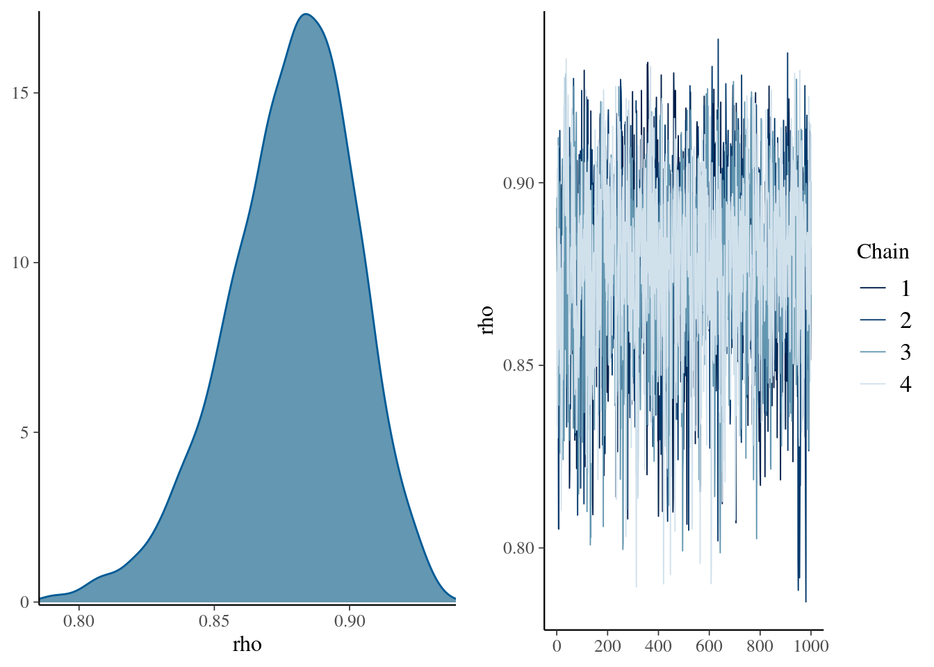
)
The Bayesian Robust Correlation: computing the Savage-Dickey density ratio
Until know the model was based on non-informative distributions, and our conclusions can be based on Credible Intervals (a.k.a Equally-Tailed Intervals), or in High Posterior Density Intervals.
But what we can do to compute Bayes Factors?
Among the simplest solutions, we can use the Savage-Dickey density ratio.
Savage-Dickey Density Ratio: the ratio between the density distributions of the posterior distribution and the prior distribution, with \(\theta = 0\). Savage-Dickey’s \(BF_{01} = Pr(\theta = 0 | D, H_0) / Pr(\theta = 0 | H_0)\)
The idea is the following:
Assuming that our \(H_0\) distribution is distributed around our “null” value (usually the zero), this should have the peak exactly on that value (otherwise, our null distribution is not a null distribution).
plot(
  y = dnorm(x = seq(from = -10, to = 10, by = 0.01)),
  x = seq(from = -10, to = 10, by = 0.01),
  type = "l",
  ylim = c(0, 0.6)
)
abline(v = 0)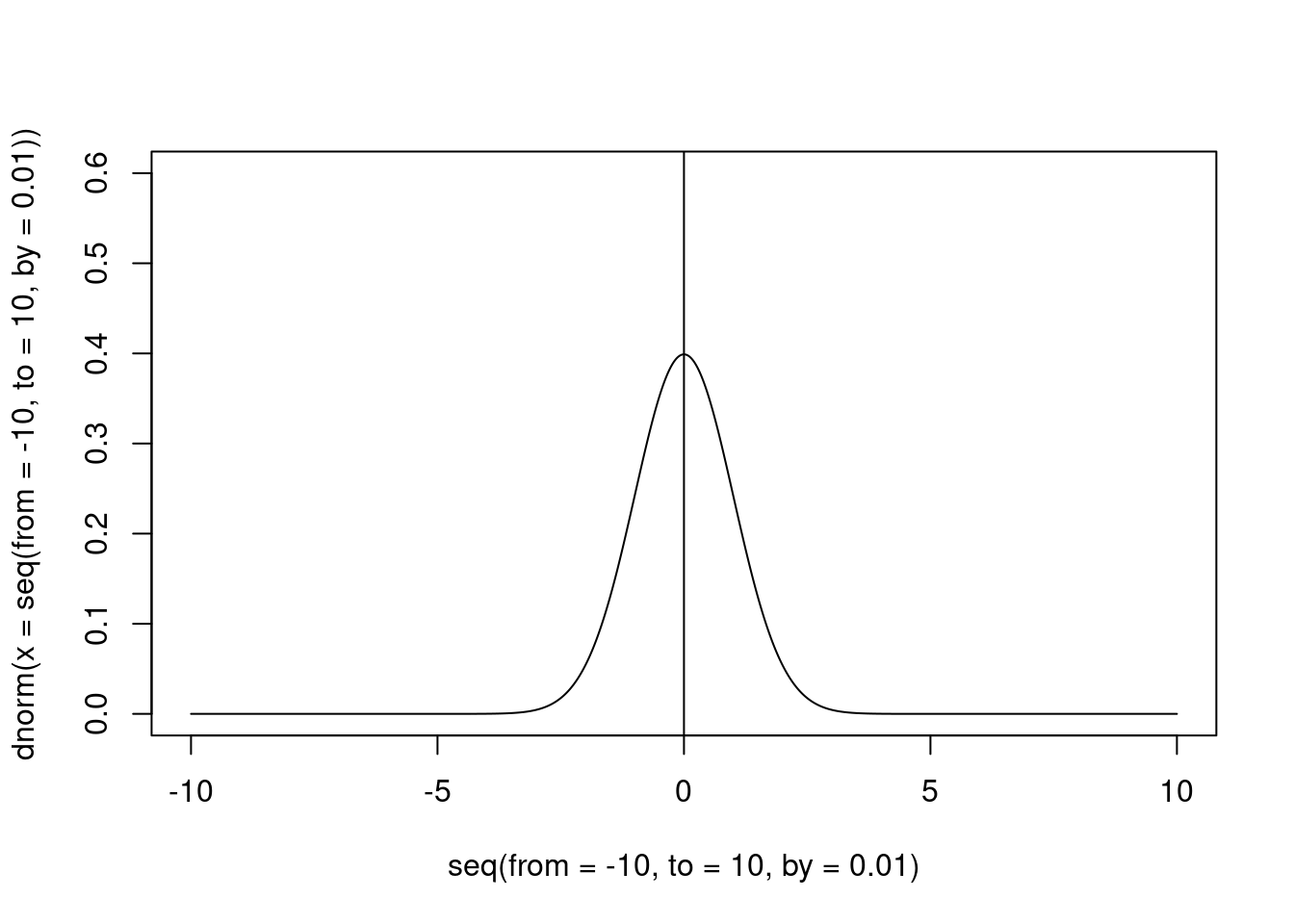
Figure 2: An example of informative prior for the null hypothesis
If our data are not distributed according our \(H_0\) distribution, the peak of the posterior distribution should be elsewhere, and the elevation of the posterior distribution at the “null” value should be less than the peak at the same position for the \(H_0\) distribution.
plot(
  y = dnorm(x = seq(from = -10, to = 10, by = 0.01)),
  x = seq(from = -10, to = 10, by = 0.01),
  type = "l",
  ylim = c(0, 0.6)
)
points(
  y = dnorm(x = seq(from = -10, to = 10, by = 0.01),
            mean = -2, sd = 2),
  x = seq(from = -10, to = 10, by = 0.01),
  col = "red",
  type = "l"
)
abline(v = 0)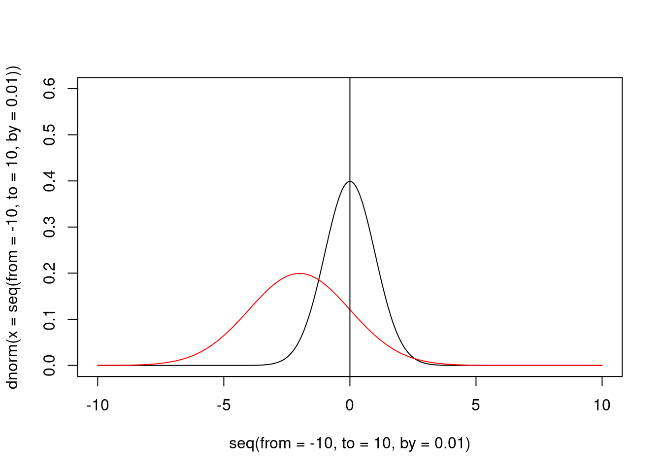
Figure 3: The prior and the posterior (red) distribution
In this case, the Savage-Dickey \(BF_{01}\) is 0.3, that is obviously in favour of the alternative hypothesis.
However, to compute the \(BF_{10}\) we could compute the reciprocal: 3.3.
OK. So far, so good.
As you have already noticed, we cannot rely anymore on non-informative prior distributions, at least for the \(\rho\) parameter.
Now, we should think to the possible informative prior for the correlation.
A natural candidate is the Beta distribution (\(\mathcal{B}(\alpha, \beta) \rightarrow [0,1]\)):
plot(
  y = dbeta(x = seq(from = 0, to = 1, by = 0.01),
            shape1 = 3, shape2 = 3),
  x = seq(from = 0, to = 1, by = 0.01),
  type = "l"
)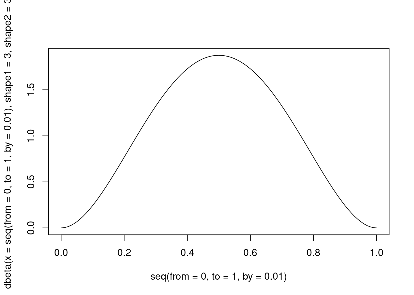
Figure 4: A Beta distribution with alpha and beta = 3
but we should stretch it in order to have a [-1, 1] range.
plot(
  y = dbeta(x = seq(from = 0, to = 1, by = 0.01),
            shape1 = 3, shape2 = 3),
  x = (seq(from = 0, to = 1, by = 0.01) - 0.5) * 2,
  type = "l"
)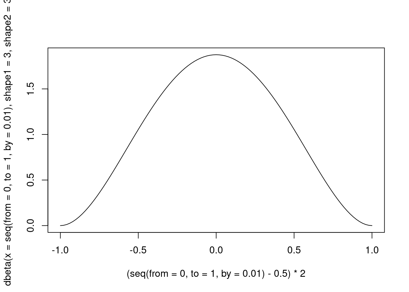
Figure 5: A Beta distribution with alpha and beta = 3
Therefore, what we will do is to use a Beta distribution, with the two parameters equal to 3, in order to have high density when \(\theta\) is equal to the “null” value. For a \(\mathcal{B}\) distribution this value is not 0, but 0.5, because this probability distribution is defined in \([0,1]\), and not in \([-\inf, +\inf]\), as it happens in distributions such as the Student’s t and the Gaussian ones.
Therefore, in the code below, I have declared the rh variable in the parameters
block, set its prior distribution as a \(\mathcal{B}(3,3)\) in the model block,
and converted it in the rho parameter, necessary to compute the
cov matrix in the transformed parameters block, necessary for the
multiple Student’s t distribution.
Finally, I have computed the \(BF_{10}\) on the rh parameter,
with a \(\theta = 0.5\), while we can use the rho parameter to get
Credible Intervals and all these statistics.
\(BF_{10} = \frac{Pr(\theta = 0.5 | D, H_0 = \mathcal{B}(\alpha = 3, \beta = 3))}{Pr(\theta = 0.5 | H_0 = \mathcal{B}(\alpha = 3, \beta = 3))}\)
library(logspline)

stancode4 <-"
data {
    int<lower=1> N;  // number of observations
    vector[2] x[N];  // input data: rows are observations, columns are the two variables
}

parameters {
    vector[2] mu;                 // locations of the marginal t distributions
    real<lower=0> sigma[2];       // scales of the marginal t distributions
    real<lower=1> nu;             // degrees of freedom of the marginal t distributions
    real<lower=0, upper=1> rh;  // correlation coefficient
}

transformed parameters {
    //correlation index rh is scaled to be within -1 and 1
    real<lower=-1, upper=1> rho = 2*(rh-0.5);
    // Covariance matrix
    cov_matrix[2] cov = [[      sigma[1] ^ 2       , sigma[1] * sigma[2] * rho],
                         [sigma[1] * sigma[2] * rho,       sigma[2] ^ 2       ]];
}

model {
    // Likelihood
    // Bivariate Student's t-distribution instead of normal for robustness
    x ~ multi_student_t(nu, mu, cov);

    // Noninformative priors on all parameters
    sigma ~ normal(0, 1000);
    mu ~ normal(0, 1000);
    nu ~ uniform(0, 1000);
    rh ~ beta(3, 3);//non informative prior between 0 and 1
}

generated quantities {
    // Random samples from the estimated bivariate t-distribution (for assessment of fit)
    vector[2] x_rand;
    x_rand = multi_student_t_rng(nu, mu, cov);
}
"

mdlCor4 <- stan(
  model_code = stancode4,
  data = data.list,
  pars = c("rho","rh"),
  refresh = 0
)
## Trying to compile a simple C file## Running /usr/lib/R/bin/R CMD SHLIB foo.c
## gcc -std=gnu99 -I"/usr/share/R/include" -DNDEBUG -I"/home/michele/R/x86_64-pc-linux-gnu-library/4.0/Rcpp/include/" -I"/home/michele/R/x86_64-pc-linux-gnu-library/4.0/RcppEigen/include/" -I"/home/michele/R/x86_64-pc-linux-gnu-library/4.0/RcppEigen/include/unsupported" -I"/home/michele/R/x86_64-pc-linux-gnu-library/4.0/BH/include" -I"/home/michele/R/x86_64-pc-linux-gnu-library/4.0/StanHeaders/include/src/" -I"/home/michele/R/x86_64-pc-linux-gnu-library/4.0/StanHeaders/include/" -I"/home/michele/R/x86_64-pc-linux-gnu-library/4.0/RcppParallel/include/" -I"/home/michele/R/x86_64-pc-linux-gnu-library/4.0/rstan/include" -DEIGEN_NO_DEBUG -DBOOST_DISABLE_ASSERTS -DBOOST_PENDING_INTEGER_LOG2_HPP -DSTAN_THREADS -DBOOST_NO_AUTO_PTR -include '/home/michele/R/x86_64-pc-linux-gnu-library/4.0/StanHeaders/include/stan/math/prim/mat/fun/Eigen.hpp' -D_REENTRANT -DRCPP_PARALLEL_USE_TBB=1 -fpic -g -O2 -fdebug-prefix-map=/build/r-base-8T8CYO/r-base-4.0.3=. -fstack-protector-strong -Wformat -Werror=format-security -Wdate-time -D_FORTIFY_SOURCE=2 -g -c foo.c -o foo.o
## In file included from /home/michele/R/x86_64-pc-linux-gnu-library/4.0/RcppEigen/include/Eigen/Core:88,
## from /home/michele/R/x86_64-pc-linux-gnu-library/4.0/RcppEigen/include/Eigen/Dense:1,
## from /home/michele/R/x86_64-pc-linux-gnu-library/4.0/StanHeaders/include/stan/math/prim/mat/fun/Eigen.hpp:13,
## from <command-line>:
## /home/michele/R/x86_64-pc-linux-gnu-library/4.0/RcppEigen/include/Eigen/src/Core/util/Macros.h:613:1: error: unknown type name ‘namespace’
## 613 | namespace Eigen {
## | ^~~~~~~~~
## /home/michele/R/x86_64-pc-linux-gnu-library/4.0/RcppEigen/include/Eigen/src/Core/util/Macros.h:613:17: error: expected ‘=’, ‘,’, ‘;’, ‘asm’ or ‘__attribute__’ before ‘{’ token
## 613 | namespace Eigen {
## | ^
## In file included from /home/michele/R/x86_64-pc-linux-gnu-library/4.0/RcppEigen/include/Eigen/Dense:1,
## from /home/michele/R/x86_64-pc-linux-gnu-library/4.0/StanHeaders/include/stan/math/prim/mat/fun/Eigen.hpp:13,
## from <command-line>:
## /home/michele/R/x86_64-pc-linux-gnu-library/4.0/RcppEigen/include/Eigen/Core:96:10: fatal error: complex: File o directory non esistente
## 96 | #include <complex>
## | ^~~~~~~~~
## compilation terminated.
## make: *** [/usr/lib/R/etc/Makeconf:172: foo.o] Errore 1## Warning: There were 3264 divergent transitions after warmup. See
## http://mc-stan.org/misc/warnings.html#divergent-transitions-after-warmup
## to find out why this is a problem and how to eliminate them.## Warning: Examine the pairs() plot to diagnose sampling problems## Warning: Bulk Effective Samples Size (ESS) is too low, indicating posterior means and medians may be unreliable.
## Running the chains for more iterations may help. See
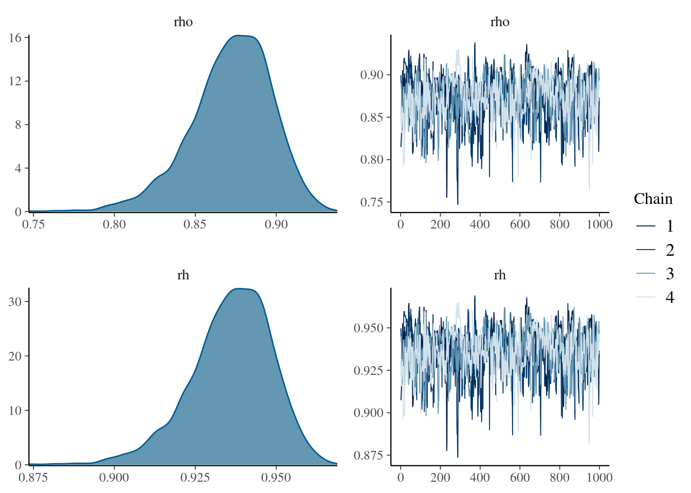
## http://mc-stan.org/misc/warnings.html#bulk-esskable( summary(mdlCor4)[[1]] , digits = 3,
caption = "Posterior distribution for the rho and rh parameters")| mean | se_mean | sd | 2.5% | 25% | 50% | 75% | 97.5% | n_eff | Rhat | |
|---|---|---|---|---|---|---|---|---|---|---|
| rho | 0.872 | 0.002 | 0.025 | 0.815 | 0.857 | 0.874 | 0.890 | 0.915 | 260.699 | 1.022 |
| rh | 0.936 | 0.001 | 0.013 | 0.907 | 0.929 | 0.937 | 0.945 | 0.957 | 260.699 | 1.022 |
| lp__ | -368.320 | 0.078 | 1.792 | -372.699 | -369.292 | -368.046 | -366.987 | -365.741 | 529.762 | 1.007 |
mcmc_combo(
  mdlCor4,
  pars = c("rho", "rh")
)
rh_logspl <- logspline( extract( mdlCor4 , pars = "rh") )## Warning in logspline(extract(mdlCor4, pars = "rh")): too much data close
## together## Warning in logspline(extract(mdlCor4, pars = "rh")): re-ran with oldlogsplineBF10 <- dbeta(0.5, 3, 3) / dlogspline(0.5, rh_logspl)The \(BF_{10} =\) 1.198786910^{26}.
This is the version with unknown degrees of freedom download the Stan code
Version with degrees of freedom coming from the sample size download the Stan code
Version with a Multi Normal distribution instead of a Multi Student’s t distribution (normal correlation) download the Stan code
The Bayesian Robust Correlation: multiple correlations
OK, I hope that everything was clear until this point.
Now, I had to compute correlations among 15 different questionnaires, that means 119 correlations.
It is true that the codes I showed you until now are pretty fast, but… the PC would have worked for days!
Therefore I prepared a version for multiple correlations.
- The Multi - something distributions can take 2 or N vectors. So this should not be a problem
- The messy thing could be the covariance matrix. I should find a more convenient way to compute it.
- Am I sure that I want to do a robust correlation? The No U-Turn Chains used in Stan are great, but adding parameters to estimate can lead to difficulties in the computations. Therefore, I would avoid a version with unknown \(\nu\)
Fortunately, in Stan there is a convenient distribution that is a sort of generalisation of the \(\mathcal{B}\) distribution, whose values are \([-1, 1]\).
This distribution is the LKJ distribution,
that has only one parameter \(\eta\) and it is marginally distributed along a
\(\mathcal{B}(\alpha, \beta)\), where \((\alpha, \beta) = \eta - 1 + K / 2\) and
\(K\) being the number of variables to be correlated.
Because correlations matrix are very important also for (Generalised) Multilevel Linear Models, in Stan there are specific distributions and variable types helping us to easy the task.
cholesky_factor_corris a variable type, it helps in creating triangular matrices perfect for correlation matrices.lkj_corr_choleskyis a prior distribution for correlationsmulti_normal_choleskyis a prior distribution for multi normal distributions, accepting a lower triangular covariation matrix instead of a covariance matrix
Now, the covariance matrix and the correlation matrix are computed in the
generate quantities block, together with the random sampling from the
distribution for posterior predictive checking.
This is done because, instead that extrapolate the cholesky matrices, it is easier to take our decisions by observing them.
set.seed(5)
## let's add an uncorrelated variable to our data set
dat$z <- rnorm( nrow(dat) )

data.list <- list(
  x = dat,
  N = nrow(dat),
  V = ncol(dat)## number of variable to be correlated
)


stancode5 <- "
data {
    int<lower=1> N;  // number of observations
    int<lower=2> V;  // number of variables
    vector[V] x[N];  // input data: rows are observations, columns are the V variables
}

parameters {
    vector[V] mu;                           // locations of the normal distributions
    vector<lower=0>[V] sigma;               // scales of the normal distributions
    cholesky_factor_corr[V] Lrho;           // correlation matrix
}

model {
    // Noninformative priors on all parameters
    target += uniform_lpdf(sigma | 0, 10);
    target += normal_lpdf(mu | 0, 10);
    target += lkj_corr_cholesky_lpdf(Lrho| 3);

    // Likelihood
    // Multivariate Normal distribution
    target += multi_normal_cholesky_lpdf(x | mu, diag_pre_multiply(sigma, Lrho));
}

generated quantities {
  matrix[V,V] Omega;
  matrix[V,V] cov;
  vector[V] x_rand;

  Omega = multiply_lower_tri_self_transpose(Lrho);
  cov = quad_form_diag(Omega, sigma);

  x_rand = multi_normal_rng(mu, cov);
}
"

mdlCor5 <- stan(
  model_code = stancode5,
  data = data.list,
  pars = "Omega",
  refresh = 0
)
## Trying to compile a simple C file## Running /usr/lib/R/bin/R CMD SHLIB foo.c
## gcc -std=gnu99 -I"/usr/share/R/include" -DNDEBUG -I"/home/michele/R/x86_64-pc-linux-gnu-library/4.0/Rcpp/include/" -I"/home/michele/R/x86_64-pc-linux-gnu-library/4.0/RcppEigen/include/" -I"/home/michele/R/x86_64-pc-linux-gnu-library/4.0/RcppEigen/include/unsupported" -I"/home/michele/R/x86_64-pc-linux-gnu-library/4.0/BH/include" -I"/home/michele/R/x86_64-pc-linux-gnu-library/4.0/StanHeaders/include/src/" -I"/home/michele/R/x86_64-pc-linux-gnu-library/4.0/StanHeaders/include/" -I"/home/michele/R/x86_64-pc-linux-gnu-library/4.0/RcppParallel/include/" -I"/home/michele/R/x86_64-pc-linux-gnu-library/4.0/rstan/include" -DEIGEN_NO_DEBUG -DBOOST_DISABLE_ASSERTS -DBOOST_PENDING_INTEGER_LOG2_HPP -DSTAN_THREADS -DBOOST_NO_AUTO_PTR -include '/home/michele/R/x86_64-pc-linux-gnu-library/4.0/StanHeaders/include/stan/math/prim/mat/fun/Eigen.hpp' -D_REENTRANT -DRCPP_PARALLEL_USE_TBB=1 -fpic -g -O2 -fdebug-prefix-map=/build/r-base-8T8CYO/r-base-4.0.3=. -fstack-protector-strong -Wformat -Werror=format-security -Wdate-time -D_FORTIFY_SOURCE=2 -g -c foo.c -o foo.o
## In file included from /home/michele/R/x86_64-pc-linux-gnu-library/4.0/RcppEigen/include/Eigen/Core:88,
## from /home/michele/R/x86_64-pc-linux-gnu-library/4.0/RcppEigen/include/Eigen/Dense:1,
## from /home/michele/R/x86_64-pc-linux-gnu-library/4.0/StanHeaders/include/stan/math/prim/mat/fun/Eigen.hpp:13,
## from <command-line>:
## /home/michele/R/x86_64-pc-linux-gnu-library/4.0/RcppEigen/include/Eigen/src/Core/util/Macros.h:613:1: error: unknown type name ‘namespace’
## 613 | namespace Eigen {
## | ^~~~~~~~~
## /home/michele/R/x86_64-pc-linux-gnu-library/4.0/RcppEigen/include/Eigen/src/Core/util/Macros.h:613:17: error: expected ‘=’, ‘,’, ‘;’, ‘asm’ or ‘__attribute__’ before ‘{’ token
## 613 | namespace Eigen {
## | ^
## In file included from /home/michele/R/x86_64-pc-linux-gnu-library/4.0/RcppEigen/include/Eigen/Dense:1,
## from /home/michele/R/x86_64-pc-linux-gnu-library/4.0/StanHeaders/include/stan/math/prim/mat/fun/Eigen.hpp:13,
## from <command-line>:
## /home/michele/R/x86_64-pc-linux-gnu-library/4.0/RcppEigen/include/Eigen/Core:96:10: fatal error: complex: File o directory non esistente
## 96 | #include <complex>
## | ^~~~~~~~~
## compilation terminated.
## make: *** [/usr/lib/R/etc/Makeconf:172: foo.o] Errore 1kable( summary(mdlCor5)[[1]] , digits = 3,
caption = "Posterior distribution for the rho parameters (Omega matrix)")| mean | se_mean | sd | 2.5% | 25% | 50% | 75% | 97.5% | n_eff | Rhat | |
|---|---|---|---|---|---|---|---|---|---|---|
| Omega[1,1] | 1.000 | NaN | 0.000 | 1.000 | 1.000 | 1.000 | 1.000 | 1.000 | NaN | NaN |
| Omega[1,2] | 0.868 | 0.000 | 0.025 | 0.815 | 0.853 | 0.870 | 0.886 | 0.910 | 3231.915 | 1.000 |
| Omega[1,3] | 0.063 | 0.001 | 0.094 | -0.127 | -0.004 | 0.066 | 0.127 | 0.245 | 4149.647 | 1.000 |
| Omega[2,1] | 0.868 | 0.000 | 0.025 | 0.815 | 0.853 | 0.870 | 0.886 | 0.910 | 3231.915 | 1.000 |
| Omega[2,2] | 1.000 | NaN | 0.000 | 1.000 | 1.000 | 1.000 | 1.000 | 1.000 | NaN | NaN |
| Omega[2,3] | 0.106 | 0.001 | 0.094 | -0.084 | 0.041 | 0.106 | 0.169 | 0.291 | 4283.671 | 1.000 |
| Omega[3,1] | 0.063 | 0.001 | 0.094 | -0.127 | -0.004 | 0.066 | 0.127 | 0.245 | 4149.647 | 1.000 |
| Omega[3,2] | 0.106 | 0.001 | 0.094 | -0.084 | 0.041 | 0.106 | 0.169 | 0.291 | 4283.671 | 1.000 |
| Omega[3,3] | 1.000 | 0.000 | 0.000 | 1.000 | 1.000 | 1.000 | 1.000 | 1.000 | 3680.380 | 0.999 |
| lp__ | -640.094 | 0.050 | 2.123 | -644.979 | -641.351 | -639.759 | -638.544 | -636.963 | 1767.064 | 1.002 |
mcmc_combo(
  mdlCor5,
  regex_pars = "Omega"
)
## Warning in regularize.values(x, y, ties, missing(ties), na.rm = na.rm):
## collapsing to unique 'x' values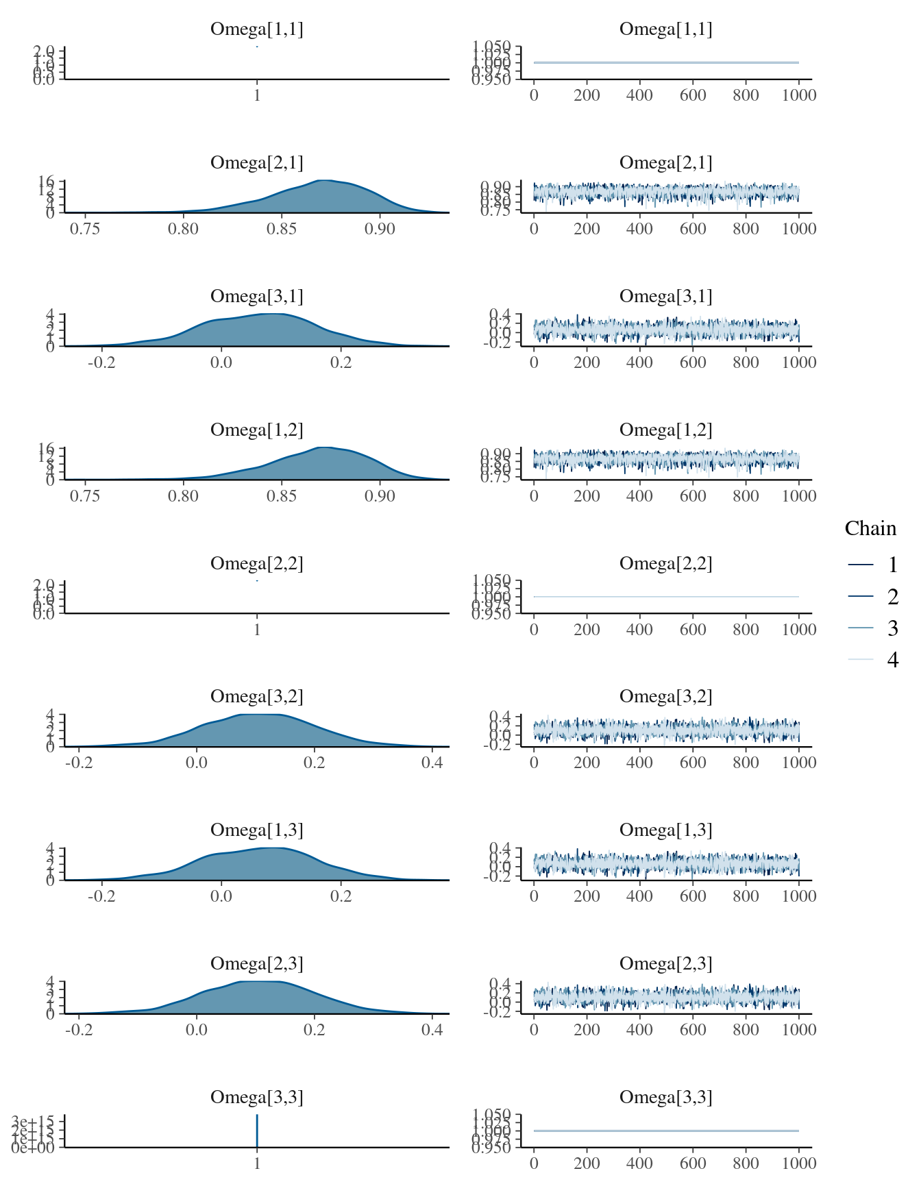
rrho <- extract( mdlCor5 , pars = "Omega")$Omega
x_rho <- rrho[ , 2:3, 1]# cor(x,y) and cor(x,z)
y_rho <- rrho[ ,   3, 2]# cor(y,z)

out <- as.data.frame(cbind(x_rho, y_rho))
colnames(out) <- c("cor(x,y)", "cor(x,z)", "cor(y,z)")

rho_logspl <- apply(out, 2, logspline)
## to understand what is eta and why we are computing it in this way,
## see some lines above where it is written
## about the LKJ distribution
## eta        <- 3 + 1 - ncol(dat)/2
BF10       <- lapply(rho_logspl,
                     FUN = function(x, eta){
                       dbeta(0.5, eta, eta) / dlogspline(0 , x)
                       },
                     eta = 3 + 1 - ncol(dat)/2
                     )

kable(do.call("c", BF10), digits = 2, caption = "The Savage-Dickey BFs")| x | |
|---|---|
| cor(x,y) | 1.583335e+21 |
| cor(x,z) | 5.200000e-01 |
| cor(y,z) | 7.700000e-01 |
Do not worry for the NaNs in the summary of the posterior distribution.
This is normal when a variable in a MCMC takes always the same value, in this case 1, because it is the correlation between a values and itself.
Remember that in the Omega matrix 1 is the x variable, 2 the y and
3 the z one.
The Bayesian Robust Correlation: multiple correlations
So let’s try to use a Student’s t-test distribution.
The \(\nu\) parameter will be the number of observations, divided by 10.
Because there is not a “cholensky” version of the multi Student’s t distribution, we should use the normal one, by passing as a parameter the covariance matrix.
For this reason, the correlation and covariance matrices are now computed in the transformed parameters block.
stancode6 <- "
data {
    int<lower=1> N;  // number of observations
    int<lower=2> V;  // number of variables
    vector[V] x[N];  // input data: rows are observations, columns are the V variables
}

parameters {
    vector[V] mu;                           // locations of the normal distributions
    vector<lower=0>[V] sigma;               // scales of the normal distributions
    cholesky_factor_corr[V] Lrho;           // correlation matrix
}

transformed parameters {
    matrix[V,V] Omega;
    matrix[V,V] cov;
    // degrees of freedom of the marginal t distributions
    real<lower=1> nu = (N / 10.0) + 1;

    // Correlation and Covariance matrices
    Omega = multiply_lower_tri_self_transpose(Lrho);
    cov   = quad_form_diag(Omega, sigma);
}

model {
    // Noninformative priors on all parameters
    target += uniform_lpdf(sigma | 0, 10);
    target += normal_lpdf(mu | 0, 10);
    target += lkj_corr_cholesky_lpdf(Lrho| 3);

    // Likelihood
    // Multivariate Student's t distribution
    target += multi_student_t_lpdf(x | nu, mu, cov);
}

generated quantities {
  vector[V] x_rand;

  x_rand = multi_student_t_rng(nu, mu, cov);
}
"

mdlCor6 <- stan(
  model_code = stancode6,
  data = data.list,
  pars = "Omega",
  refresh = 0
)
## Trying to compile a simple C file## Running /usr/lib/R/bin/R CMD SHLIB foo.c
## gcc -std=gnu99 -I"/usr/share/R/include" -DNDEBUG -I"/home/michele/R/x86_64-pc-linux-gnu-library/4.0/Rcpp/include/" -I"/home/michele/R/x86_64-pc-linux-gnu-library/4.0/RcppEigen/include/" -I"/home/michele/R/x86_64-pc-linux-gnu-library/4.0/RcppEigen/include/unsupported" -I"/home/michele/R/x86_64-pc-linux-gnu-library/4.0/BH/include" -I"/home/michele/R/x86_64-pc-linux-gnu-library/4.0/StanHeaders/include/src/" -I"/home/michele/R/x86_64-pc-linux-gnu-library/4.0/StanHeaders/include/" -I"/home/michele/R/x86_64-pc-linux-gnu-library/4.0/RcppParallel/include/" -I"/home/michele/R/x86_64-pc-linux-gnu-library/4.0/rstan/include" -DEIGEN_NO_DEBUG -DBOOST_DISABLE_ASSERTS -DBOOST_PENDING_INTEGER_LOG2_HPP -DSTAN_THREADS -DBOOST_NO_AUTO_PTR -include '/home/michele/R/x86_64-pc-linux-gnu-library/4.0/StanHeaders/include/stan/math/prim/mat/fun/Eigen.hpp' -D_REENTRANT -DRCPP_PARALLEL_USE_TBB=1 -fpic -g -O2 -fdebug-prefix-map=/build/r-base-8T8CYO/r-base-4.0.3=. -fstack-protector-strong -Wformat -Werror=format-security -Wdate-time -D_FORTIFY_SOURCE=2 -g -c foo.c -o foo.o
## In file included from /home/michele/R/x86_64-pc-linux-gnu-library/4.0/RcppEigen/include/Eigen/Core:88,
## from /home/michele/R/x86_64-pc-linux-gnu-library/4.0/RcppEigen/include/Eigen/Dense:1,
## from /home/michele/R/x86_64-pc-linux-gnu-library/4.0/StanHeaders/include/stan/math/prim/mat/fun/Eigen.hpp:13,
## from <command-line>:
## /home/michele/R/x86_64-pc-linux-gnu-library/4.0/RcppEigen/include/Eigen/src/Core/util/Macros.h:613:1: error: unknown type name ‘namespace’
## 613 | namespace Eigen {
## | ^~~~~~~~~
## /home/michele/R/x86_64-pc-linux-gnu-library/4.0/RcppEigen/include/Eigen/src/Core/util/Macros.h:613:17: error: expected ‘=’, ‘,’, ‘;’, ‘asm’ or ‘__attribute__’ before ‘{’ token
## 613 | namespace Eigen {
## | ^
## In file included from /home/michele/R/x86_64-pc-linux-gnu-library/4.0/RcppEigen/include/Eigen/Dense:1,
## from /home/michele/R/x86_64-pc-linux-gnu-library/4.0/StanHeaders/include/stan/math/prim/mat/fun/Eigen.hpp:13,
## from <command-line>:
## /home/michele/R/x86_64-pc-linux-gnu-library/4.0/RcppEigen/include/Eigen/Core:96:10: fatal error: complex: File o directory non esistente
## 96 | #include <complex>
## | ^~~~~~~~~
## compilation terminated.
## make: *** [/usr/lib/R/etc/Makeconf:172: foo.o] Errore 1kable( summary(mdlCor6)[[1]] , digits = 3,
caption = "Posterior distribution for the rho parameters (Omega matrix)")| mean | se_mean | sd | 2.5% | 25% | 50% | 75% | 97.5% | n_eff | Rhat | |
|---|---|---|---|---|---|---|---|---|---|---|
| Omega[1,1] | 1.000 | NaN | 0.000 | 1.000 | 1.000 | 1.000 | 1.000 | 1.000 | NaN | NaN |
| Omega[1,2] | 0.863 | 0.000 | 0.027 | 0.803 | 0.846 | 0.866 | 0.882 | 0.909 | 3155.376 | 1.000 |
| Omega[1,3] | 0.094 | 0.002 | 0.100 | -0.101 | 0.029 | 0.094 | 0.160 | 0.286 | 4016.328 | 0.999 |
| Omega[2,1] | 0.863 | 0.000 | 0.027 | 0.803 | 0.846 | 0.866 | 0.882 | 0.909 | 3155.376 | 1.000 |
| Omega[2,2] | 1.000 | NaN | 0.000 | 1.000 | 1.000 | 1.000 | 1.000 | 1.000 | NaN | NaN |
| Omega[2,3] | 0.130 | 0.002 | 0.099 | -0.065 | 0.062 | 0.131 | 0.196 | 0.323 | 4304.939 | 0.999 |
| Omega[3,1] | 0.094 | 0.002 | 0.100 | -0.101 | 0.029 | 0.094 | 0.160 | 0.286 | 4016.328 | 0.999 |
| Omega[3,2] | 0.130 | 0.002 | 0.099 | -0.065 | 0.062 | 0.131 | 0.196 | 0.323 | 4304.939 | 0.999 |
| Omega[3,3] | 1.000 | 0.000 | 0.000 | 1.000 | 1.000 | 1.000 | 1.000 | 1.000 | 3894.519 | 0.999 |
| lp__ | -644.844 | 0.052 | 2.151 | -649.951 | -646.086 | -644.445 | -643.278 | -641.624 | 1737.786 | 1.000 |
mcmc_combo(
  mdlCor6,
  regex_pars = "Omega"
)
## Warning in regularize.values(x, y, ties, missing(ties), na.rm = na.rm):
## collapsing to unique 'x' values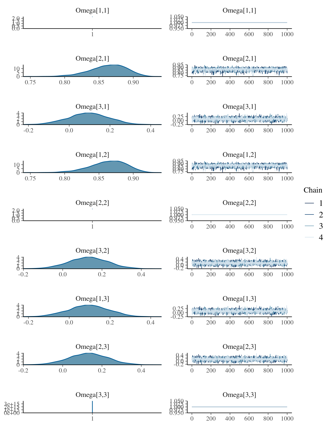
rrho <- extract( mdlCor6 , pars = "Omega")$Omega
x_rho <- rrho[ , 2:3, 1]# cor(x,y) and cor(x,z)
y_rho <- rrho[ ,   3, 2]# cor(y,z)

out <- as.data.frame(cbind(x_rho, y_rho))
colnames(out) <- c("cor(x,y)", "cor(x,z)", "cor(y,z)")

rho_logspl <- apply(out, 2, logspline)

BF10       <- lapply(rho_logspl,
                     FUN = function(x, eta){
                       dbeta(0.5, eta, eta) / dlogspline(0 , x)
                       },
                     eta = 3 + 1 - ncol(dat)/2
                     )

kable(do.call("c", BF10), digits = 2, caption = "The Savage-Dickey BFs")| x | |
|---|---|
| cor(x,y) | 1.046782e+22 |
| cor(x,z) | 6.500000e-01 |
| cor(y,z) | 1.020000e+00 |
Conclusions
We have seen how to compute Bayesian correlations using Stan.
What we are actually doing, is to model a covariance matrix among all the observed variables, and extracting the correlations from it.
I have spent a little time in explaining what to do for using robust correlations (that do not have an equivalent in the frequentist framework), how to compute Savage-Dickey ratios from them, and how to use this framework for multiple correlations.
Actually, the versions for multiple correlations are faster than the versions for the correlations between two only variables, because they are not using ugly conversions of the \(\mathcal{B}(\alpha,\beta)\) distribution, but they use the more convenient LKJ distributions.
If you are not interested in computing the Savage-Dickey ratio, and you would
like to have a non-informative distribution for the correlations (i.e.,
\(\mathcal{U}(-1, 1)\)), you just need to change
target += lkj_corr_cholesky_lpdf(Lrho| 3);
in target += lkj_corr_cholesky_lpdf(Lrho| 1);, that is equivalent to
\(\mathcal{U}(-1, 1)\), but more powerful.
Would you like to learn something more about Bayesian Statistics?
There are a lot of excellent books and tutorials online, but if you want to have an overall overview of the main aspects, you might be interested in a Summer School, such as the BayesHSC Summer School that will be held on-line or in Verona, from May \(31^{st}\) to June \(5^{th}\), 2021.
We are looking forward for you!